Source apportionment and driving factor identification for typical watersheds soil heavy metals of tibetan plateau based on receptor models and geodetector

ABSTRACT The identification and quantification of soil heavy metal (HM) pollution sources and the identification of driving factors is a prerequisite of soil pollution control. In this

paper, the Sabaochaqu Basin of the Tuotuo River, located in the Tibetan Plateau and the headwater of the Yangtze River, was selected as the study area. The soil pollution was evaluated using

geochemical baseline, and the source apportionment of soil HMs was performed using absolute principal component score-multiple linear regression (APCS-MLR), edge analysis (UNMIX) and

positive matrix decomposition (PMF). The driver of the source factor was identified with the geodetector method (GDM). The results of pollution evaluation showed that the HM pollution of

soil in the study area was relatively light. By comparison, UNMIX model was considered to be the preferred model for soil HMs quantitative distribution in this study area, followed by PMF

model. The UNMIX model results show that source 1 (U-S1) was dominated by As, with a contribution rate of 53.31%; source 2 (U-S2) was dominated by Cd and Zn, whose contribution rates are

50.35% and 46.60% respectively; source 3 (U-S3) was dominated by Pb, with a contribution rate of 45.58%; source 4 (U-S4) was dominated by Cr, Cu, Hg and Ni, with contribution rates of

60.58%, 60.07%, 51.58% and 56.45%, respectively. The GDM results showed that the main driving factors of U-S1 were distance from lake (explanatory power q = 0.328) and distance from wind

channel (q = 0.168), which were defined as long-distance migration sources. The main driving factors of U-S2 were parent material type (q = 0.269) and distance from Tuotuo river (q = 0.213),

which were defined as freeze-thaw sources. The main driving factors of U-S3 were distance from town (q = 0.255) and distance from county road (Yanya Line) (q = 0.221), which were defined as

human activity sources. The main drivers of U-S4 were V (q = 0.346) and Sc (q = 0.323), which were defined as natural sources. The GDM results of the 3 models were generally consistent with

the analytical results of similar types of sources, especially the results of PMF model and Unmix model can basically verify each other. The research results can provide important

theoretical reference for the analysis of HM sources in the soil of high-cold and high-altitude regions. SIMILAR CONTENT BEING VIEWED BY OTHERS SOURCE IDENTIFICATION AND DRIVING FACTOR

APPORTIONMENT FOR SOIL POTENTIALLY TOXIC ELEMENTS VIA COMBINING APCS-MLR, UNMIX, PMF AND GDM Article Open access 13 May 2024 SOURCE APPORTIONMENT OF SOIL HEAVY METALS WITH PMF MODEL AND PB

ISOTOPES IN AN INTERMOUNTAIN BASIN OF TIANSHAN MOUNTAINS, CHINA Article Open access 12 November 2022 SOURCE ANALYSIS OF HEAVY METAL POLLUTION IN AGRICULTURAL SOIL IRRIGATED WITH SEWAGE IN

WUQING, TIANJIN Article Open access 08 September 2021 INTRODUCTION Heavy metal (HM) elements mainly include Pb, Hg, Sb, Cr, Cd, Co, Ni, Cu, etc., as well as the metalloid element As and its

compounds. HMs exist widely in soil environment, with the characteristics of difficult degradation, lasting harm, irreversible and food chain accumulation1,2, and the pollution caused by

them has aroused long-term concern in the world. Soil HM pollution is more prominent in some areas of China. According to the national soil pollution survey, the exceedance rate of soil Cd,

Hg, As, Cu, Pb, Cr, Zn and Ni sample points were 7.0%, 1.6%, 2.7%, 2.1%, 1.5%, 1.1%, 0.9% and 4.8%, respectively3. The first step to prevent and control soil HM pollution is to identify the

source of HMs4. Therefore, to explore the sources and driving factors of HMs in soil is a hot issue in the study of HM pollution5,6,7. China’s “Opinions of the CPC Central Committee and The

State Council on Comprehensively Promoting the Construction of a Beautiful China” issued on January 11, 2024 also stressed the need to carry out soil pollution source prevention and control

actions, and promote the traceability of agricultural land soil heavy metal pollution and full coverage of remediation in stages. Single factor pollution index (PI) and composite pollution

index (SPI) are important indexes used to assess the level of HM pollution in soil8. Since PI and SPI should be evaluated with background values as reference standards, the earth’s crust

element content, national soil element background value, provincial and municipal regional background value, comparative value of adjacent regions or historical data are usually used as

reference standards for evaluation. However, due to the different geological characteristics and human environment in different regions, using a uniform reference standard to evaluate soil

HM pollution may lead to inaccurate evaluation results9,10. The use of geochemical baseline as a reference standard can represent the concentration of HMs in soil that is not affected by

human beings, and can objectively assess the level of soil pollution11. Receptor model is a multivariate statistical method, which has been widely used in the source identification of

pollutants, and is considered as an important tool to prevent and control soil HM pollution12,13,14,15. Among many receptor models, absolute principal component analysis-multiple linear

regression (APCS-MLR), UNMIX model, and positive definite matrix decomposition (PMF) model were widely used because they can perform source identification while input environmental

observations into the model16. APCS-MLR obtained absolute factor score and quantitative contribution of each source factor by regression and multiple linear regression. The UNMIX model

determines the number of source factors by singular value decomposition, and then calculates the contribution of source factors by self-modeling curve decomposition technology. The PMF

calculates the contribution of each source factor and its corresponding uncertainty based on the concentration of HMs in each soil sample17. Due to the different algorithms and mechanisms

used by different receptor models, their quantitative source identify results of soil HMs may be different. Therefore, different models should be used for analysis of the same data set at

the same time to obtain more reasonable source factors15,17,18. However, these receptor models all have some common shortcomings, such as the inability to consider the spatial changes of

data, the inability to analyze categorical variable such as land use type and soil type, and the source factors analyzed should be defined by existing knowledge, which is obviously

subjective17. Geo-detector is a statistical method to detect spatial differentiation and reveal the driving factors behind it19,20, which can make up for the shortcomings of these receptor

models. The influence of the impact factors on soil HMs can be explained in detail through the geo-detector3,21,22. Based on the characteristics of the geo-detector, the geographical

detector can be used to explain the influence of the impact factors on the source factors resolved by the receptor model, and the source factors can be accurately analyzed and defined

through the difference of influence. Therefore, this study took the Sabaochaqu basin of the Tuotuo River, located in the Tibetan Plateau and the headwater of the Yangtze River, as the

research area to determine the geochemical baseline of soil HMs, and used this as the reference standard to evaluate the pollution level of soil HMs. Three receptor models (APCS-MLR, UNMIX

and PMF) were used to quantitatively identify the source factors of HMs. Combined with the geo-detector to accurately identify the driving factors of each source factor, the soil HM sources

in this area can be more reasonably explained, which makes up for the deficiency of soil HM studies in the Tuotuo River basin at the source of the Yangtze River, and provides a theoretical

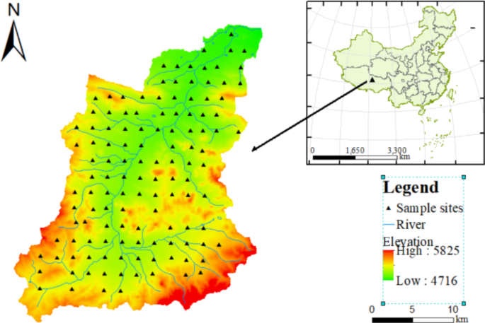
reference for the apportionment of soil HM sources in the high-cold and high-altitude regions. MATERIALS AND METHODS STUDY AREA The study area is located in the hinterland of the Tibetan

plateau, the northernmost part of Anduo county, Tibet (90°32°47.62”-91°49°13.06” E, 33°23°16.46”-34°41°31.47” N) (Fig. 1). The climate belongs to the excessive zone of cold, semi-arid and

semi-humid climate, which is an alpine steppe ecosystem with cold and dry, thin air, strong wind, open terrain, and high wind speed under the influence of cold air activity near the ground

and strong westerly wind from the sky. The annual average number of gale days is more than 110 days. The temperature and pressure are low, the temperature difference between day and night is

large, and the radiation is strong. The freezing period is from September to April of the following year. The annual average pressure is 584.3mb, and the annual average temperature is

-4.2℃. The lowest altitude of the study area is 4716 m, the highest is 5825 m, and the high-altitude area is mainly distributed in the southwest and southeast of the study area. The natural

environment in the study area is harsh and rainfall is less. SAMPLING AND ANALYSIS Field sampling to be completed in 2022. A total of 128 pieces of topsoil (0–20 cm) were collected according

to the 1:250000 land quality geochemical evaluation specification. The sampling locations were shown in Fig. 1. In order to improve the representativeness of soil samples, the sampling

points were uniformly arranged in a 4 km² sampling grid, and the distance between each sampling point was required to be greater than 2 km. 3–5 multi-point collections within 100 m around

the sampling point are combined into one sample, and the original weight of the combined sample is greater than 1 kg. The sampling locations were recorded by GPS. Remove visible impurities

from all collected samples and air-dried at room temperature. The analysis and testing were completed by Chengdu Comprehensive Rock and Mineral Testing Center of Sichuan Provincial Bureau of

Geology and Mineral Exploration and Development. pH was measured by ion selective electrode method (for water extraction without carbon dioxide, the ratio of soil to water was 1/2.5), Corg

was measured by volumetric method (analysis methods for regional geochemical sample-part 27: determination of organic carbon contents by potassium dichromate volumetric method (DZ/T 0279.

27-2016)). N was measured by combustion infrared method (analysis methods for regional geochemical sample-part 29: determination of nitrogen contents by Kjeldahl distillation-volumetric

method (DZ/T 0279. 29-2016)). As and Hg were measured by atomic fluorescence method (methods for chemical analysis of silicate rocks-part 33: determination of arsenic, stibium, bismuth and

mercury elements content-hydride generation atomic fluorescence spectrometry (GB/T 14506.33–2019)). V, Cu, Pb, Zn, Ni, Cr, Cd and Sc were measured by X-ray Fluorescence (analysis methods for

regional geochemical sample-part 1: determination of 24 components including aluminum oxide etc. by pressed power pellets-X-ray fluorescence spectrometry (DZ/T 0279. 1-2016)), inductively

coupled plasma mass spectrometry (analysis methods for regional geochemical sample-part 3: determination of 15 elements including barium, beryllium, bismuth etc. by inductively coupled

plasma mass spectrometry (DZ/T 0279. 3-2016)) and inductively coupled plasma optical emission spectrometer (analysis methods for regional geochemical sample-part 2: determination of 27

components including calcium oxide etc. by inductively coupled plasma atomic emission spectrometry (DZ/T 0279. 2-2016)). The quality of analysis and testing was controlled by means of

inserting national first-level soil standard materials, repeatability inspection, abnormal point inspection and blank test. GEOCHEMICAL BASELINE Firstly, the average value

(\(\:\stackrel{-}{\text{X}}\)) and standard deviation (σ) of the initial data set are calculated, and the values beyond the range of \(\:\stackrel{-}{\text{X}}\)±2σ are eliminated. Repeat

this step for the new data set until all the residual values are in the range of \(\:\stackrel{-}{\text{X}}\)±2σ, and the remaining data sets conform to normal distribution or lognormal

distribution. The arithmetic mean value or geometric mean value of the final retained data is used as the geochemical baseline value, respectively23,24. POLLUTION INDEX METHOD The pollution

index method includes single factor pollution index (PI) and comprehensive pollution index (SPI). PI is based on the total amount of single HM in a single soil, which can simply and

effectively evaluate the pollution degree caused by single HM in a single soil. SPI can effectively reflect the comprehensive pollution degree of different HMs to the soil environment, and

its calculation formula is shown in the literature25,26. It is divided into 5 pollution levels according to PI and SPI: clean (< 0.7), alert (0.7-1.0), light pollution (1.0–2.0), medium

pollution (2.0–3.0) and heavy pollution (≥ 3.0). RECEPTOR MODELS APCS-MLR MODEL The APCS-MLR model was proposed by Thurston and Spengler in 1985. Which can determine the load of HMs to each

pollution source, and calculate the average contribution of each source to soil HMs. The detailed steps are as follows:

$$\:{Z}_{ij}=\frac{{C}_{ij}-\stackrel{-}{C}}{{\sigma\:}_{j}}\:\:\:\:\:\:\:\:\:\:\:\:\:\:\:\:$$ (1)

$$\:{{(Z}_{0})}_{j}=\frac{0-\stackrel{-}{{C}_{j}}}{{\sigma\:}_{j}}=-\frac{\stackrel{-}{{C}_{j}}}{{\sigma\:}_{j}}\:\:\:\:\:\:\:\:\:\:\:\:\:\:\:\:\:\:\:\:\:\:\:\:\:\:\:\:\:\:\:\:\:\:\:\:\:\:\:\:\:\:\:\:\:\:\:\:\:\:\:\:\:\:\:\:\:\:\:\:\:\:$$

(2) $$\:{\text{X}}_{\text{i}}={\text{b}}_{0}+\sum\:_{\text{k}=1}^{\text{m}}{\text{b}}_{\text{k}}{\text{A}\text{P}\text{C}\text{S}}_{\text{k}}$$ (3) where, C_ij_ is the concentration of

_jth_ type in _ith_ sample; and \(\:\stackrel{-}{{C}_{j}}\) and \(\:{\upsigma\:}\)_j_ are the arithmetic average concentration and standard deviation for _jth_ type, respectively. b0 is the

intercept of regression for soil HM, bk is the regression coefficient of the soil HM, m is the number of factors, APCSk is the adjusted score of the _k_th source, bkAPCSk can be regarded as

the contribution of the _k_th source to the soil HM concentrations. UNMIX MODEL In this model, the data space dimensionality is reduced via singular value decomposition, and then number of

sources, source composition and contribution rate of sources of each sample can be estimated (USEPA, 2007). The fundamental model can be characterized as follow:

$$\:{C}_{ij}=\sum\:_{k=1}^{m}{U}_{ik}{D}_{kj}+{S}_{ij}$$ (4) where Cij is the concentrations of _b_th HMs in _i_th sample, Uik is the contribution of _k_th in the _i_th sample, Dkj is the

concentrations of the _j_th HMs from _k_th source, Sij is the error. The source component spectrum parsed by the model needs to meet minimum system requirements that can be interpreted by

the model (Min R2 > 0.8, Min Sig/Noise > 2). PMF MODEL The PMF model decomposed the original matrix Xij into two factor matrices gik and fkj as well as a residual matrix eij, and it

was expressed as follows (USEPA, 2014):

$$\:{\text{x}}_{\text{i}\text{j}}=\sum\:_{\text{k}=1}^{\text{p}}{\text{g}}_{\text{i}\text{k}}{\text{f}}_{\text{k}\text{j}}+{\text{e}}_{\text{i}\text{j}}$$ (5) where, _x__i_j is the

concentration of the _j_th HM in the _i_th sample (mg/kg); _g__ik_ is the contribution of the _k_th source in the _i_th sample; _f__kj_ is the concentrations of the _j_th HM from the _k_th

source factor; and _e__ij_ is the residual. The residual error matrix eij is calculated by the minimum value of the objective function Q calculated according to the Eq. (9):

$$\:\text{Q}=\sum\:_{i=1}^{n}\sum\:_{j=1}^{m}{\left[\frac{{e}_{ij}}{{u}_{ij}}\right]}^{2}\:\:\:\:\:\:\:\:\:\:\:\:\:\:\:\:\:\:\:\:\:\:\:\:\:\:\:\:\:\:\:\:\:\:\:\:\:\:\:\:\:\:\:\:\:\:\:\:\:\:\:\:$$

(6) where uij is the uncertainty of the _j_th HMs in _i_th samples. The uncertainty (u) of the HMs was calculated as follows27: For c_ij_≤dij:

$$\:{x}_{ij}=\frac{{d}_{ij}}{2},\:{u}_{ij}=\frac{{d}_{ij}}{2}$$ (7) For c_ij_> dij: $$\:{x}_{ij}={c}_{ij}$$ (8) if \(\:{x}_{ij}\le\:\) 3\(\:\:{d}_{ij}\),

$$\:{u}_{ij}=\frac{{d}_{ij}}{3}+0.2\times\:{c}_{ij}$$ (9) if \(\:{x}_{ij}>\) 3\(\:\:{d}_{ij}\), $$\:{u}_{ij}=\frac{{d}_{ij}}{3}+0.1\times\:{c}_{ij}$$ (10) For missing values:

$$\:{x}_{ij}=\stackrel{-}{{c}_{ij}}\:,\:{u}_{ij}=4\stackrel{-}{{c}_{ij}}$$ (11) where xij is the concentration of sample species, dij is the detection limit, σij is the xij concentration

uncertainty, cij is the sample measured concentration, \(\:\stackrel{-}{{c}_{ij}}\)is the measured concentrations geometric mean. GEO-DETECTOR METHOD (GDM) GDM was an effective tool to

analyze the spatial variance that can identify the explanatory variables affecting the dependent variable based on the assumption that explanatory variable (X) is associated with dependent

variable (Y) if their spatial pattern is consistent20. The detailed calculation references20. The dependent variables are the mean factor scores of APCS-MLR and PMF, 21 explanatory variables

including distance from other rivers (except Tuotuo river) (DFOR), distance from town (DFT), distance from wind channel (DFWC), distance to roads within the research area (DWRA), distance

from railway (DFR), distance from National Highway G109 (DFNH), distance from County Road (Yanya Line) (DFCR), distance from Tuotuo river (DFTR), distance from lake (DFL), elevation (ELE),

NDVI, slope direction (SD), slope (SL), land vegetation type (LVT), erosion type (ET), parent material type (PMT), organic carbon (Corg), soil N content (N), soil Sc content (Sc), soil pH

value (pH) and soil V content (V). If the independent variable was numerical quantity, it needs to be discretized into type quantity20. The natural breakpoint method was used to divide 21

influencing factors into 10 categories. GeoDetector (http://www.geodetector.org/) SPSS26.0, ArcGIS10.8 and Origin2019 were used in this study. Table 1 listed the abbreviations of the

manuscript’s proper nouns. RESULTS AND DISCUSSION DESCRIPTION OF SOIL HMS IN STUDY AREA The descriptive statistics of 126 surface soil samples from the study area were shown in Table 2. The

arithmetic average contents of As, Cd, Cr, Cu, Hg, Ni, Pb, and Zn were 31.8, 0.29, 66.1, 17.4, 0.021, 27.9, 49.4 and 88.6 mg/kg, respectively. The Kolmogorov-Smirnov normality test showed

that Cr and Ni were normally distributed, and Pb had a lognormal normal distribution, and As, Cd, Cu, Hg and Zn were skewed. Except for Cr and Ni, the coefficients of variation were more

than 30%, among which As, Cd, Pb and Zn were more than 50%, which showed that there was obvious spatial heterogeneity of soil HMs, implying that there were some geographical differences and

some anthropogenic perturbations in the content of these HMs in the soils of the study area. GEOCHEMICAL BASELINES Taking As as an example (Fig. 2), the mean ± 2σ was used to continuously

remove the outliers in the initial data set of soil HM content, and the Kolmogorov-Smirnov test was performed on the data subset formed after iteration. The results showed that As, Cr and Cu

were normally distributed, and the baseline values were represented by the arithmetic mean. Cd, Hg, Ni, Pb, and Zn follow a lognormal distribution, with a geometric mean representing the

baseline value. Therefore, the baseline values of As, Cd, Cr, Cu, Hg, Ni, Pb and Zn were 22.42, 0.204, 65.06, 15.85, 0.0184, 26.39, 34.90 and 68.60 mg/kg, respectively. SOIL HMS

CONTAMINATION DISTRIBUTION CHARACTERISTICS The distribution characteristics of PI and SPI based on environmental geochemical baseline values as reference standards were shown in Fig. 3. The

PI values of As, Cd, Cr, Cu, Hg, Ni, Pb and Zn ranged from 0.41 to 7.00, 0.63–10.69, 0.55–1.69, 0.54–5.50, 0.46–3.59, 0.51–1.83, 0.56–16.73 and 1.29–8.48, respectively. The average PI values

of the 8 HMs in descending order were as follows: Cd(1.44) ≈ As(1.42) ≈ Pb(1.41) > Zn(1.29) > Hg(1.16) > Cu(1.09) ≈ Ni(1.06) > Cr(1.02), which means that the 8 HMs in the study

area were light pollution (1.0–2.0). The comprehensive pollution index (SPI) of the 8 HMs ranged from 0.84 to 12.28, with an average value of 1.77, showing a light pollution (1.0–2.0) level

overall. For the pollution distribution, Cr and Ni light pollution areas were mainly distributed in the northwest, south, southwest and central regions; The mildly polluted areas of Cu and

Hg were concentrated in the other regions except the northeast and central part of the study area, and the moderately and severely polluted areas of Cu and Hg appeared in the western corner,

while the moderately and severely polluted areas of Hg appeared in the southwest corner. As and Cd were mildly polluted in most areas of the study area, and the area of moderate and severe

pollution was large, mainly concentrated in the southern and central areas. In addition to the northwest of the region, the Pb pollution was basically light or above, and the moderate and

severe pollution areas were mainly concentrated in the south and east. In addition to the northern regions, Zn basically showed mild and above pollution, and the moderate and severe

pollution areas were mainly concentrated in the south. SPI was at light pollution level and above except for a few regions in the northeast and the north, and moderate and heavy pollution

areas were mainly concentrated in the south, west, southwest and central regions. SOURCE APPORTIONMENT OF SOIL HMS SOURCE APPORTIONMENT OF APCS-MLR MODEL KMO and Bartlett sphericity tests

for soil HMs in showed that KMO was 0.620, generally, KMO greater than 0.6 is suitable for factor analysis, The significance in Bartlett sphericity test was 0.000 it is assumed that the

significance level is 0.001, and the probability value P of the sample in this paper is lower than 0.001, so the sample is suitable for factor analysis28. APCS-MLR model was used to extract

four source factors (Fig. 4(a)), which covered 84.935% of the total variance of interpretation and could explain most of the information of HMs. Source 1 (A-S1), source 2 (A-S2), source 3

(A-S3) and source 4 (A-S4) accounted for 27.209%, 26.322%, 18.801% and 12.603% of the total variance respectively. The determination coefficients R2 of As, Cd, Cr, Cu, Hg, Ni, Pb and Zn were

0.963, 0.784, 0.773, 0.763, 0.757, 0.860, 0.917 and 0.939, respectively, all above 0.75. R2 is used to measure the correlation between the model and the actual observed value, the value is

closer to 1, the higher the linear fit and the better the simulation result29. In source apportionment, soil HMs with high load can be used as the typical HMs of the source factor17. A-S1

has the highest loading of Pb with a contribution of 50.70%, and Zn also has a higher loading with a contribution of 22.09%. A-S2 was mainly dominated by Cd, Cr, Cu, Ni and Zn, with

contributions of 49.62%, 88.86%, 73.11%, 93.62%, and 58.13%, respectively, and additionally, As, Hg, and Pb were also present in this source factor with a large loadings of 34.90%, 27.27%

and 24.50%, respectively. A-S3 was mainly dominated by Hg, with a contribution rate of 64.88%, followed by Cd, Cu and Pb, which also existed with high contribution rates of 37.50%, 22.18%

and 20.48%, respectively. A-S4 was mainly dominated by As, with a contribution rate of 56.41%. SOURCE APPORTIONMENT OF UNMIX MODEL Figure 4(b) shows the source apportionment results of UNMIX

6.0 software, in which 4 source factors (U-S1, U-S2, U-S3 and U-S4) were extracted. Min R2 = 0.95, indicating that 95% of species variance can be explained by the model, which was greater

than the minimum value required by the system (min R2 > 0.8), min(S/N) = 2.32, which was greater than the minimum value required by the system (min(S/N) > 2), it can be seen that the

analytic results obtained by the UNMIX model were credible17. The determination coefficients R2 of As, Cd, Cr, Cu, Hg, Ni, Pb and Zn were 0.84, 0.89, 0.94, 0.95, 0.97, 0.99, 0.99 and 0.99,

respectively, all above 0.8. The dominant HMs of U-S1 was As, and the contribution rate was 53.31%. The dominant HMs of U-S2 were Cd and Zn, the contribution rates are 50.35% and 46.60%,

respectively. The dominant HMs of U-S3 was Pb, the contribution rate was 45.58%; The dominant HMs of U-S4 were Cr, Cu, Hg and Ni, with contribution rates of 60.58%, 60.07%, 51.58% and

56.45%, respectively. SOURCE APPORTIONMENT OF PMF MODEL Figure 4(c) shows the source apportionment results of EPA PMF 5.0 software, and also extracts four source factors (P-S1, P-S2, P-S3,

and P-S4). The signal-to-noise ratio (S/N) of all HMs measured by PMF was above 4, indicating that the data quality was strong30. The determination coefficients R2 of As, Cd, Cr, Cu, Hg, Ni,

Pb and Zn were 0.995, 0.934, 0.779, 0.864, 0.433, 0.787, 0.995 and 0.871, respectively, and the R2 of Hg was relatively low. P-S1 was dominated by Cr, Cu, Hg and Ni, with contribution rates

of 60.28%, 63.32%, 48.99% and 60.90%, respectively. P-S2 was dominated by Pb, and the contribution rate was 47.81%. P-S3 was dominated by As, with a contribution rate of 63.84%; P-S4 were

dominated by Cd and Zn, contributing 47.63% and 37.26% respectively. COMPARISON OF THREE MODELS The accuracy of different models can be judged by comparing the determination coefficient17.

In this study, comparing the R2 values of the three models, it was found that the R2 value range of 8 HMs in the UNMIX model was the best, ranging from 0.84 to 0.99, indicating that the HM

source factors obtained by UNMIX model had the highest accuracy. The second model was APCS-MLR, with R2 values ranging from 0.757 to 0.963. The R2 value of PMF model was poor, ranging from

0.433 to 0.995, which may be caused by the sensitivity of PMF model to outliers31. In order to explain the relationship between the source apportionment factors of the same model and the

relationship between the source factors obtained by different models, Pearson correlation analysis was performed on the source apportionment results of the three models, and the results were

shown in Fig. 5. For the 4 source factors obtained by the APCS-MRL model, A-S3 and A-S4 had a very significant (_P_ < 0.01) positive correlation, and the R2 was 0.42, which meant that

the source apportionment factors A-S3 and A-S4 obtained by the model were not completely separated. There was no significant positive correlation between the 4 source factors obtained by

UNMIX model, and similar results are obtained by PMF model, indicating that the source factor separation effect obtained by the two models were better. Comparing the source factors obtained

by the 3 models, there were extremely significant or significant positive correlations among A-S1, U-S2 and P-S4, A-S2, U-S4 and P-S1, and between A-S4, U-S1 and P-S3, as well as between

U-S3 and P-S2, which means that the analytical results of the 3 models for similar types of sources were basically the same, and their results can be verified with each other15. That is,

A-S1, U-S2 and P-S4 may be a class of source factors, A-S2, U-S4 and P-S1 may be a class of source factors, A-S4, U-S1 and P-S3 may be a class of source factors, U-S3 and P-S2 may be a class

of source factors. However, A-S3 has significant positive correlation with U-S2, P-S3 and P-S4, and A-S4 and P-S3 also show significant correlation, which further confirms the conclusion

that source factors A-S3 and A-S4 were not completely separated in the APCS-MLR model. In general. UNMIX model was considered to be the first choice for soil HMs quantitative apportionment

in this study area, followed by PMF model, and APCS-MLR model was relatively poor. GDM IDENTIFY SOURCE FACTOR DRIVERS The q value of GDM was used to quantify the influence of each influence

factor on the source factor obtained by the 3 models. The largest q value influence factor indicates that the influence factor was the dominant explanatory variable. DRIVERS OF SOURCE

FACTORS FOR UNMIX MODEL APPORTIONMENT Figure 6 shows the GDM results of the 4 source factors (U-S1, U-S2, U-S3, and U-S4) analyzed by the Unmix model with 21 influence factors. The U-S1 was

dominated by DFL (q = 0.328), followed by DFWC (q = 0.168), which indicates that the lakes in the study area have a very significant influence on U-S1. In addition, long-distance

transportation also has an important influence on U-S1. Guo et al.32 pointed out that HMs in lake sediments of the Qinghai-Tibet Plateau were greatly affected by soil and atmospheric

sedimentation in the basin. Zhu et al.33 analyzed pollutants in lake sediments in the southern Qinghai-Tibet Plateau and found that the proportion of pollutants released by glacial meltwater

was 40-61%, which was corresponding to climate warming. With climate change, the degradation of the cryosphere (glaciers, permafrost, ice and snow) releases pollutants from meltwater into

lakes, and then migrates to the surrounding soil through evaporation, runoff transport and other behaviors34,35,36. It can be seen that climate warming may promote the secondary release of

pollutants from glaciers and permafrost to the atmosphere, discharge with meltwater, and other processes. Although the Himalayas in the south of the Qinghai-Tibet Plateau hinder atmospheric

transport, the transport of HMs cannot be completely blocked37. Peak-valley wind patterns may facilitate trans-Himalayan transport of pollutants38. Atmospheric circulation patterns also

affect remote plateau areas39. For example, Cong et al.40 pointed out that South Asia may be the source region of HM pollutants in atmospheric particulate matter in Namtso; Zhang et al.41

pointed out that Pb and Zn in Qinghai Lake atmospheric particulate matter samples were affected by the long-distance migration of winds from eastern China. Overall, U-S1 can be defined as a

long-distance migration source. U-S2 was dominated by PMT (q = 0.269), followed by DFTR (q = 0.213), which means that the soil parent material type and lake in the study area have a very

significant influence on U-S2. There were great differences in the composition of different types of soil parent materials, arsenic-rich rocks such as shale were widely distributed in the

Qinghai-Tibet Plateau42, Tibet soils developed from ultramafic rocks were usually rich in Ni and Co43, and the weathering products of basic bedrock may be the main source of most HMs in

Tibet soils1. The enrichment characteristics of HMs in soils formed by different parent materials were quite different. When soils undergo freeze-thaw process, due to the different parent

materials, the physical and chemical properties of soil aggregates, porosity and bulk density were also quite different, and the HM pollutants released were also significantly different.

Therefore, U-S2 can be defined as a freeze-thaw source. U-S3 was dominated by DFT (q = 0.255), followed by DFCR (q = 0.221), which indicates that road traffic activities and human activities

were the main driving factors of U-S3. In this study, the contribution rate of Pb to U-S3 was the largest (45.58%) (Fig. 4 (b)), and the coefficient of variation of Pb was the largest

(106.6%), indicating that human activities strongly influenced the accumulation of Pb in soil. Previous studies have shown that Pb was mainly derived from traffic emissions, such as exhaust

from leaded gasoline, erosion of engine brakes, and catalytic combustion44. In the Tibetan Plateau, the burning of yak manure has a significant impact on the atmospheric HMs content45. Kang

et al.46 found that the average daily concentration of Pb in TSP increased to 81.39ng/m3 when nomads in Namtso used cow dung for cooking or heating in tents. In addition, fireworks, garbage

burning, traffic, and religious ceremonies all lead to an increase in the concentration of HMs in the surrounding air45, which migrates and settles into the soil. According to the pollution

distribution characteristics (Fig. 3), the areas with high Pb pollution were mainly concentrated in the southern and southeastern regions closer to Maqu Township. In summary, U-S3 can be

defined as a source of human activity. The results of GDM showed that V (q = 0.346) and Sc (q = 0.323) were dominant in U-S4. In this study, Cr, Cu, Hg and Ni had the largest contribution to

U-S4 (Fig. 4 (b)), but their coefficients of variation were all less than 50% (Table 2), showing similar pollution distribution characteristics (Fig. 3), and their PI values showed

relatively lowest pollution, which confirmed that the concentrations of soil Cr, Cu, Hg and Ni in the study area were dependent on natural sources. Therefore, U-S4 can be defined as a

natural source. DRIVERS OF SOURCE FACTORS FOR APCS-MLR AND PMF MODELS APPORTIONMENT Figure 7 lists the two factors that have the greatest GDM explanatory power of the source factors A-S1,

A-S2, A-S3, A-S4, P-S1, P-S2, P-S3 and P-S4 obtained by APCS-MLR and PMF models apportionment. The main driving factors of A-S2 and P-S1 were consistent with the main driving factors of

U-S4, which were crustal elements Sc and V. The results of correlation analysis also show that there was a significant correlation among them (Fig. 5), which means that A-S2 and P-S1 were

natural sources like U-S4. The main driving factors of A-S1 were DFNH (q = 0.147) and DFR (q = 0.139), and the main driving factors of P-S2 were DFT (q = 0.237) and DFNH (q = 0.231). The

main driving factors of both were similar to the main driving factors of U-S3. In comparison with the results of correlation analysis, A-S1, P-S2 and U-S3 all have significant correlations,

and the largest contribution rate was Pb, so A-S1 and P-S2 belong to human activity sources like U-S3. Correlation analysis indicated that A-S3 and A-S4 were not completely separated, and

GDM results showed that the influence factor DFWC had a significant impact on A-S3 and A-S4, which further confirmed the conclusion of correlation analysis. The main driving factors of A-S4

and P-S3 were DFL and DFWC, which were consistent with the main driving factors of U-S1, and the contribution rate of the three source factors were mainly from the heavy metal As. In

addition, there was a very significant correlation among them, which means that A-S4, P-S3 and U-S1 were consistent with long-distance migration sources. The main driving factors of P-S4 and

U-S2 were similar, and the correlation coefficient was 0.86. It indicates that P-S4 and U-S2 belong to the same class source and were freeze-thaw sources. Generally speaking, the GDM

results of the three models were basically the same for similar types of sources, especially the results of PMF model and Unmix model can basically verify each other. By running different

models and verifying the results, the applicability of different models in soil HM source distribution in the study area was verified. Due to the different algorithms used by different

models, the results of source allocation were both similar and different. Therefore, different models should be used for source analysis, which can enhance the persuasiveness of the results.

MEANING OF MULTI-SOURCE INTERPRETATION Using effective tools to identify and quantify soil HMs source contribution was of great significance for soil HMs pollution source prevention and

control, pollution tracing and control, but PI, SPI, enrichment factor, accumulation index and other methods were not enough to identify and quantify the source contribution of soil HMs.

Therefore, the comprehensive application of receptor model, correlation analysis and GDM can effectively identify and quantify the source of soil HMs. The receptor model does not need to

collect emission inventory information, but quantifies the HMS source distribution characteristics according to the spatial distribution characteristics of soil HMs17,47. However, the source

factors obtained from the receptor model were explained based on a priori knowledge of previous studies and experiences. In order to further explain the source factors derived from the

receptor model, this study uses the GDM method to identify the driving factors of source factors by examining the spatial correlation between source factors and pollution impact factors. The

results of GDM can help explain the source of each source factor obtained from the receptor model. In this study, the contents of soil Sc and V are taken as natural sources, the distance

from the sampling point to the road and township represents the source of human activity, the distance from the sampling point to the distant wind channel represents the long-distance

migration source, and the distance from the sampling point to lakes and rivers represents the freezing and thawing source. Generally speaking, this comprehensive method can better understand

the various pollution sources of soil HMs and better define the source factors, which is of great significance for the local control of soil HMs in the study area, and can also provide an

important theoretical reference for the analysis of soil HM sources in high-cold and high-altitude areas. CONCLUSIONS With the rapid development of the global economy and the intensification

of global warming, the pollution of HMs in soils in high-cold and high-altitude areas such as the Qinghai-Tibet Plateau has become increasingly prominent. In this study, three receptor

models were combined with correlation analysis and GDM to quantitatively analyze the source factors and driving factors of soil HMs in typical watersheds of Qinghai-Tibetan Plateau. Unmix

model can well fit the observed-predicted values of HMs in most soils in the study area, and it is an ideal receptor model, followed by PMF model. The analytical results of the three models

for similar types of sources were basically the same, and their results can be verified with each other. The combination of receptor model and GDM can effectively explain the four source

factors identified by receptor model, including natural source, human activity source, long-distance migration source and freeze-thaw source. In fact, the accumulation of HMs in soil was a

complex process, which was affected by a variety of environmental factors. In the next step of research, more environmental factors and analysis methods affecting soil HMs accumulation

should be considered, especially the introduction of isotope analysis to better identify long-distance migration sources and freeze-thaw sources to ensure more accurate identification. DATA

AVAILABILITY All data generated or analysed during this study are included in this published article. REFERENCES * Sheng, J. J., Wang, X. P., Gong, P., Tian, L. D. & Yao, T. D. Heavy

metals of the tibetan top soils level, source, spatial distribution, temporal variation and risk assessment. _Environ. Sci. Pollut. Res._ 19, 3362–3370.

https://doi.org/10.1007/s11356-012-0857-5 (2012). Article  CAS  Google Scholar  * Nagajyoti, P. C., Lee, K. D. & Sreekanth, T. V. M. Heavy metals, occurrence and toxicity for plants: A

review. _Environ. Chem. Lett._ 8, 199–216. https://doi.org/10.1007/s10311-010-0297-8 (2010). Article  CAS  Google Scholar  * Gong, C. et al. Spatial differentiation and influencing factor

analysis of soil heavy metal content at town level based on geographic detector. _Environ. Sci._ 43, 4566–4577. https://doi.org/10.13227/j.hjkx.202112077 (2022). Article  Google Scholar  *

Marrugo-Negrete, J., Pinedo-Hernández, J. & Díez, S. Assessment of heavy metal pollution, spatial distribution and origin in agricultural soils along the Sinu River Basin, Colombia.

_Environ. Res._ 154, 380–388. https://doi.org/10.1016/j.envres.2017.01.021 (2017). Article  CAS  PubMed  Google Scholar  * Kaige, L. et al. Development of a new method framework to estimate

the nonlinear and interaction relationship between environmental factors and soil heavy metals. _Sci. Total Environ._ 905, 167133–167133. https://doi.org/10.1016/j.scitotenv.2023.167133

(2023). Article  CAS  Google Scholar  * Chen, D. et al. Accumulation and source apportionment of soil heavy metals in molybdenum lead-zinc polymetallic ore concentration area of Luanchuan.

_Rock. Mineral. Anal._ 42, 839–851. https://doi.org/10.15898/j.ykcs.202208090147 (2023). Article  CAS  Google Scholar  * Cao, S. et al. Sources and ecological risk of heavy metals inthe

sediments of off shore area in Quanzhou Bay, Fujian Province. _Geol. China_. 49, 1481–1496 (2022). CAS  Google Scholar  * Wang, F. F. et al. Contamination characteristics, source

apportionment, and health risk assessment of heavy metals in agricultural soil in the Hexi Corridor. _Catena_ https://doi.org/10.1016/j.catena.2020.104573 (2020). * Li, M. et al. Optimizing

the soil environmental protection standard system and suggestions. _Res. Environ. Sci._ 29, 1799–1810. https://doi.org/10.13198/j.issn.1001-6929.2016.12.08 (2016). Article  Google Scholar  *

Sun, H. et al. Determination of heavy metal geochemical baseline values and its accumulation in soils of the Luanhe river basin, Chengde. _Environ. Sci._ 40, 3753–3763.

https://doi.org/10.13227/j.hjkx.201901056 (2019). Article  Google Scholar  * Galán, E., Fernández-Caliani, J. C., González, I., Aparicio, P. & Romero, A. Influence of geological setting

on geochemical baselines of trace elements in soils. Application to soils of South-West Spain. _J. Geochem. Explor._ 98, 89–106. https://doi.org/10.1016/j.gexplo.2008.01.001 (2008). Article

  CAS  Google Scholar  * Huang, J. H. et al. A new exploration of health risk assessment quantification from sources of soil heavy metals under different land use. _Environ. Pollut._ 243,

49–58. https://doi.org/10.1016/j.envpol.2018.08.038 (2018). Article  CAS  PubMed  Google Scholar  * Yang, X. et al. Source identification and comprehensive apportionment of the accumulation

of soil heavy metals by integrating pollution landscapes, pathways, and receptors. _Sci. Total Environ._ 786 https://doi.org/10.1016/j.scitotenv.2021.147436 (2021). * Wang, Y. N. et al.

Source apportionment of soil heavy metals: a new quantitative framework coupling receptor model and stable isotopic ratios. _Environ. Pollut._ 314

https://doi.org/10.1016/j.envpol.2022.120291 (2022). * Guan, Q. Y. et al. Source apportionment of heavy metals in farmland soil of Wuwei, China: comparison of three receptor models. _J.

Clean. Prod._ 237 https://doi.org/10.1016/j.jclepro.2019.117792 (2019). * Deng, J. J. et al. Source apportionment of PM2.5 at the Lin’an regional background site in China with three receptor

models. _Atmos. Res._ 202, 23–32. https://doi.org/10.1016/j.atmosres.2017.11.017 (2018). Article  CAS  Google Scholar  * Guo, G. H., Li, K., Zhang, D. G. & Lei, M. Quantitative source

apportionment and associated driving factor identification for soil potential toxicity elements via combining receptor models, SOM, and geo-detector method. _Sci. Total Environ._ 830

https://doi.org/10.1016/j.scitotenv.2022.154721 (2022). * Zhang, M. N. & Lv, J. S. Source apportionment of potentially toxic elements in soils of the Yellow River Delta Nature Reserve,

China: the application of three receptor models and geostatistical independent simulation. _Environ. Pollut._ 289 https://doi.org/10.1016/j.envpol.2021.117834 (2021). * Wang, J. F. et al.

Geographical detectors-based health risk assessment and its application in the neural tube defects study of the Heshun Region, China. _Int. J. Geogr. Inf. Sci._ 24, 107–127.

https://doi.org/10.1080/13658810802443457 (2010). Article  CAS  Google Scholar  * Wang, J. & Xu, C. Geodetector: Principle and prospective. _Acta Geogr. Sin._ 72, 116–134 (2017). Google

Scholar  * Qiao, P. W., Yang, S. C., Lei, M., Chen, T. B. & Dong, N. Quantitative analysis of the factors influencing spatial distribution of soil heavy metals based on geographical

detector. _Sci. Total Environ._ 664, 392–413. https://doi.org/10.1016/j.scitotenv.2019.01.310 (2019). Article  ADS  CAS  PubMed  Google Scholar  * Yang, Y., Yang, X., He, M. J. &

Christakos, G. Beyond mere pollution source identification: determination of land covers emitting soil heavy metals by combining PCA/APCS, GeoDetector and GIS analysis. _Catena_. 185

https://doi.org/10.1016/j.catena.2019.104297 (2020). * Wu, F., Chen, L., Yi, T., Yang, Z. & Chen, Y. Determination of heavy metal baseline values and analysis of its accumulation

characteristics in agricultural land in Chongqing. _Environ. Sci._ 39, 5116–5126. https://doi.org/10.13227/j.hjkx.201803205 (2018). Article  Google Scholar  * Li, H., Jiang, X., Wang, S.

& Che, F. Geochemical baseline establishment in grassland-type lake sediments in cold-arid regions: A case study in Dalinuoer Lake, China. _China Environ. Sci._ 42, 5803–5813.

https://doi.org/10.19674/j.cnki.issn1000-6923.20220915.003 (2022). Article  CAS  Google Scholar  * Wang, C. et al. Pollution level and risk assessment of heavy metals in a metal smelting

area of Xiong’an New District. _Geol. China_. 48, 1697–1709. https://doi.org/10.12029/gc20210603 (2021). Article  CAS  Google Scholar  * Feng, J. et al. Evaluation and migration path

analysis of soil heavy metal pollution in a metal mining area of Qinling mountain. _Rock. Mineral. Anal._ 42, 1189–1202. https://doi.org/10.15898/j.ykcs.202302170021 (2023). Article  CAS 

Google Scholar  * Zhang, J. Z. et al. Trace elements in PM < sub > 2.5 in Shandong Province: Source identification and health risk assessment. _Sci. Total Environ._ 621, 558–577.

https://doi.org/10.1016/j.scitotenv.2017.11.292 (2018). Article  ADS  CAS  PubMed  Google Scholar  * Jung, J. et al. Environmental forensic approach towards unraveling contamination sources

with receptor models: A case study in Nakdong River, South Korea. _Sci. Total Environ._ 892 https://doi.org/10.1016/j.scitotenv.2023.164554 (2023). * Li, Q. et al. Spatial distribution

characteristics and source analysis of soil heavy metals at typical smelting industry sites. _Environ. Sci._ 42, 5930–5937. https://doi.org/10.13227/j.hjkx.202104313 (2021). Article  CAS 

Google Scholar  * Sharma, S. K. et al. Chemical characterization and source apportionment of aerosol at an urban area of Central Delhi, India. _Atmos. Pollut. Res._ 7, 110–121.

https://doi.org/10.1016/j.apr.2015.08.002 (2016). Article  Google Scholar  * Jin, Z. & Lv, J. S. Integrated receptor models and multivariate geostatistical simulation for source

apportionment of potentially toxic elements in soils. _Catena_. 194 https://doi.org/10.1016/j.catena.2020.104638 (2020). * Guo, B. X., Liu, Y. Q., Zhang, F., Hou, J. Z. & Zhang, H. B.

Characteristics and risk assessment of heavy metals in core sediments from lakes of Tibet. _Environ. Sci._ 37, 490–498. https://doi.org/10.13227/j.hjkx.2016.02.012 (2016). Article  CAS 

Google Scholar  * Zhu, T. T. et al. Accumulation of pollutants in Proglacial Lake sediments: Impacts of glacial meltwater and anthropogenic activities. _Environ. Sci. Technol._ 54,

7901–7910. https://doi.org/10.1021/acs.est.0c01849 (2020). Article  ADS  CAS  PubMed  Google Scholar  * Wang, W. J. et al. Assessing sources and distribution of heavy metals in environmental

media of the Tibetan Plateau: A critical review. _Front. Environ. Sci._ 10 https://doi.org/10.3389/fenvs.2022.874635 (2022). * Zhang, S. H. et al. Analysis of heavy metal-related indices in

the Eboling permafrost on the Tibetan Plateau. _Catena_ (2021). https://doi.org/10.1016/j.catena.2020.104907 * Ci, Z. J., Peng, F., Xue, X. & Zhang, X. S. Permafrost thaw dominates

mercury emission in Tibetan thermokarst ponds. _Environ. Sci. Technol._ 54, 5456–5466. https://doi.org/10.1021/acs.est.9b06712 (2020). Article  ADS  CAS  PubMed  Google Scholar  * Wang, X.

P., Gong, P., Wang, C. F., Ren, J. & Yao, T. D. A review of current knowledge and future prospects regarding persistent organic pollutants over the Tibetan Plateau. _Sci. Total Environ._

573, 139–154. https://doi.org/10.1016/j.scitotenv.2016.08.107 (2016). Article  ADS  CAS  PubMed  Google Scholar  * Cong, Z. Y. et al. New insights into trace element wet deposition in the

Himalayas: Amounts, seasonal patterns, and implications. _Environ. Sci. Pollut. Res._ 22, 2735–2744. https://doi.org/10.1007/s11356-014-3496-1 (2015). Article  CAS  Google Scholar  * Yang,

K. et al. Recent climate changes over the Tibetan Plateau and their impacts on energy and water cycle: A review. _Glob. Planet Change_. 112, 79–91.

https://doi.org/10.1016/j.gloplacha.2013.12.001 (2014). Article  ADS  Google Scholar  * Cong, Z. Y., Kang, S. C., Liu, X. D. & Wang, G. F. Elemental composition of aerosol in the Nam Co

region, Tibetan Plateau, during summer monsoon season. _Atmos. Environ._ 41, 1180–1187. https://doi.org/10.1016/j.atmosenv.2006.09.046 (2007). Article  ADS  CAS  Google Scholar  * Zhang, N.

N. et al. Chemical composition and sources of PM < sub > 2.5 and TSP collected at Qinghai Lake during summertime. _Atmos. Res._ 138, 213–222.

https://doi.org/10.1016/j.atmosres.2013.11.016 (2014). Article  CAS  Google Scholar  * Li, C. L., Kang, S. C., Zhang, Q. G., Gao, S. P. & Sharma, C. M. Heavy metals in sediments of the

Yarlung Tsangbo and its connection with the arsenic problem in the Ganges-Brahmaputra Basin. _Environ. Geochem. Health_. 33, 23–32. https://doi.org/10.1007/s10653-010-9311-0 (2011). Article

  CAS  PubMed  Google Scholar  * Yin, A. & Harrison, T. M. Geologic evolution of the Himalayan-Tibetan orogen. _Annu. Rev. Earth Planet. Sci._ 28, 211–280.

https://doi.org/10.1146/annurev.earth.28.1.211 (2000). Article  ADS  CAS  Google Scholar  * Cai, L. M., Wang, Q. S., Wen, H. H., Luo, J. & Wang, S. Heavy metals in agricultural soils

from a typical township in Guangdong Province, China: Occurrences and spatial distribution. _Ecotox Environ. Safe_. 168, 184–191. https://doi.org/10.1016/j.ecoenv.2018.10.092 (2019). Article

  CAS  Google Scholar  * Chen, P. F., Kang, S. C., Bai, J. K., Sillanpää, M. & Li, C. L. Yak dung combustion aerosols in the Tibetan Plateau: Chemical characteristics and influence on

the local atmospheric environment. _Atmos. Res._ 156, 58–66. https://doi.org/10.1016/j.atmosres.2015.01.001 (2015). Article  CAS  Google Scholar  * Kang, S. C., Li, C. L., Wang, F. Y.,

Zhang, Q. G. & Cong, Z. Y. Total suspended particulate matter and toxic elements indoors during cooking with yak dung. _Atmos. Environ._ 43, 4243–4246.

https://doi.org/10.1016/j.atmosenv.2009.06.015 (2009). Article  ADS  CAS  Google Scholar  * PriyaDarshini, S., Sharma, M. & Singh, D. Synergy of receptor and dispersion modelling:

Quantification of PM 10 emissions from road and soil dust not included in the inventory. _Atmospheric Pollution Res._ 7, 403–411 (2016). Article  Google Scholar  Download references FUNDING

This research was supported by Geological Survey Project of China Geological Survey (DD20243076, DD20243098, DD20243127, DD20242769) and Open Foundation of the Key Laboratory of Natural

Resource Coupling Process and Effects (No. 2023KFKTB011). AUTHOR INFORMATION AUTHORS AND AFFILIATIONS * Research Center of Applied Geology of China Geological Survey, Chengdu, 610039, China

Cang Gong, Jun Tan, Weiqing Yang, Changhai Tan & Lang Wen * Key Laboratory of Natural Resource Coupling Process and Effects, Beijing, 100055, China Cang Gong, Changhai Tan, Lang Wen 

& Jiufen Liu * Natural Resources Comprehensive Survey Command Center of China Geological Survey, Beijing, 100055, China Jiufen Liu & Liming Gan * Xi’an Center of Mineral Resources

Survey, China Geological Survey, Xi’an, 710100, China Liming Gan Authors * Cang Gong View author publications You can also search for this author inPubMed Google Scholar * Jun Tan View

author publications You can also search for this author inPubMed Google Scholar * Weiqing Yang View author publications You can also search for this author inPubMed Google Scholar * Changhai

Tan View author publications You can also search for this author inPubMed Google Scholar * Lang Wen View author publications You can also search for this author inPubMed Google Scholar *

Jiufen Liu View author publications You can also search for this author inPubMed Google Scholar * Liming Gan View author publications You can also search for this author inPubMed Google

Scholar CONTRIBUTIONS Cang Gong: Conceptualization, Methodology, Formal analysis, Data Curation, Writing - Original Draft, Visualization. Changhai Tan and Lang Wen: Methodology, Software,

Formal analysis, Investigation, Data Curation. Jun Tan: Conceptualization, Writing-Review & Editing, Supervision. iufen Liu: Conceptualization, Investigation, Supervision, Writing-Review

& Editing. Liming Gan: Conceptualization, Investigation, Supervision, Writing-Review & Editing. All authors have approval to the final version of the manuscript. CORRESPONDING

AUTHORS Correspondence to Cang Gong, Jun Tan or Liming Gan. ETHICS DECLARATIONS COMPETING INTERESTS The authors declare no competing interests. ADDITIONAL INFORMATION PUBLISHER’S NOTE

Springer Nature remains neutral with regard to jurisdictional claims in published maps and institutional affiliations. RIGHTS AND PERMISSIONS OPEN ACCESS This article is licensed under a

Creative Commons Attribution-NonCommercial-NoDerivatives 4.0 International License, which permits any non-commercial use, sharing, distribution and reproduction in any medium or format, as

long as you give appropriate credit to the original author(s) and the source, provide a link to the Creative Commons licence, and indicate if you modified the licensed material. You do not

have permission under this licence to share adapted material derived from this article or parts of it. The images or other third party material in this article are included in the article’s

Creative Commons licence, unless indicated otherwise in a credit line to the material. If material is not included in the article’s Creative Commons licence and your intended use is not

permitted by statutory regulation or exceeds the permitted use, you will need to obtain permission directly from the copyright holder. To view a copy of this licence, visit

http://creativecommons.org/licenses/by-nc-nd/4.0/. Reprints and permissions ABOUT THIS ARTICLE CITE THIS ARTICLE Gong, C., Tan, J., Yang, W. _et al._ Source apportionment and driving factor

identification for typical watersheds soil heavy metals of Tibetan Plateau based on receptor models and geodetector. _Sci Rep_ 14, 29108 (2024). https://doi.org/10.1038/s41598-024-75161-2

Download citation * Received: 07 May 2024 * Accepted: 03 October 2024 * Published: 24 November 2024 * DOI: https://doi.org/10.1038/s41598-024-75161-2 SHARE THIS ARTICLE Anyone you share the

following link with will be able to read this content: Get shareable link Sorry, a shareable link is not currently available for this article. Copy to clipboard Provided by the Springer

Nature SharedIt content-sharing initiative KEYWORDS * Source apportionment * Driving factor identification * Soil heavy metals * Tibetan plateau * Receptor models * Geodetector