A comparison of deep learning U-Net architectures for posterior segment OCT retinal layer segmentation

Deep learning methods have enabled a fast, accurate and automated approach for retinal layer segmentation in posterior segment OCT images. Due to the success of semantic segmentation methods

adopting the U-Net, a wide range of variants and improvements have been developed and applied to OCT segmentation. Unfortunately, the relative performance of these methods is difficult to

ascertain for OCT retinal layer segmentation due to a lack of comprehensive comparative studies, and a lack of proper matching between networks in previous comparisons, as well as the use of

different OCT datasets between studies. In this paper, a detailed and unbiased comparison is performed between eight U-Net architecture variants across four different OCT datasets from a

range of different populations, ocular pathologies, acquisition parameters, instruments and segmentation tasks. The U-Net architecture variants evaluated include some which have not been

previously explored for OCT segmentation. Using the Dice coefficient to evaluate segmentation performance, minimal differences were noted between most of the tested architectures across the

four datasets. Using an extra convolutional layer per pooling block gave a small improvement in segmentation performance for all architectures across all four datasets. This finding

highlights the importance of careful architecture comparison (e.g. ensuring networks are matched using an equivalent number of layers) to obtain a true and unbiased performance assessment of

fully semantic models. Overall, this study demonstrates that the vanilla U-Net is sufficient for OCT retinal layer segmentation and that state-of-the-art methods and other architectural

changes are potentially unnecessary for this particular task, especially given the associated increased complexity and slower speed for the marginal performance gains observed. Given the

U-Net model and its variants represent one of the most commonly applied image segmentation methods, the consistent findings across several datasets here are likely to translate to many other

OCT datasets and studies. This will provide significant value by saving time and cost in experimentation and model development as well as reduced inference time in practice by selecting

simpler models.

Optical coherence tomography (OCT) is a non-invasive, high resolution imaging modality that is commonly used in ophthalmic imaging. By allowing easy visualisation of the retinal tissue, OCT

scans can be employed by clinicians and researchers for diagnosis of ocular diseases and monitoring disease progression or response to therapy through the quantitative and qualitative

analysis of features within these images. The inner and outer boundaries of the retinal and choroidal layers are of particular interest in OCT image analysis. However, the marking of the

position of these boundaries can be slow and inefficient when performed manually by a human expert annotator. Therefore, rapid and reliable automated algorithms are necessary to perform

retinal segmentation in a time-efficient manner.

Early automatic methods for OCT retinal and choroidal segmentation relied upon standard image processing techniques as part of methods that were handcrafted to suit particular sets of

images1,2,3,4,5,6,7,8,9. While these methods achieve the goal of saving time, the specific nature of the rules that make up their algorithms means that they may not generalise well to other

data without manually recalibrating the algorithm, which can take considerable time and present notable difficulties. On the other hand, a range of alternative methods have been proposed

which are based on deep learning. A deep learning method can automatically learn the rules from a dataset, rectifying one of the main drawbacks of traditional analysis techniques.

Additionally, extending an algorithm to new data typically requires simply extending the training set with the new samples, while most other training and model parameters do not need to be

modified for the method to operate. There are numerous deep learning methods that have been proposed for OCT retinal segmentation with a few different techniques commonly employed including

patch-based methods10,11,12,13,14 and semantic segmentation methods14,15,16,17,18,19,20,21,22,23,24,25,26, among others. Semantic segmentation methods, in particular, have demonstrated

state-of-the-art performance in retinal and choroidal layer segmentation tasks of OCT images14.

The majority of semantic segmentation methods adopt an encoder-decoder deep neural network structure, most of which base their architectures on the U-Net27, improving over the original

fully-convolutional network approach28. In the U-Net, skip connections improve gradient flow and allow the transfer of information between the down-sampling and up-sampling paths by

connecting each pair of encoder-decoder layers. The U-Net takes an input OCT image and classifies each individual pixel in the image into one of several possible classes, thereby segmenting

the image into the different regions. For OCT retinal layer segmentation, the classes correspond to the different tissue layers and other regions around the tissue layers of interest. The

output of the U-Net is a pixel-level map providing precise segmentation of the regions and layers of interest.

There are several variants which aim to improve performance compared to the original (vanilla) U-Net architecture. Dense U-Net29,30 connects all convolution block outputs to the inputs of

all subsequent blocks within each level which encourage feature reuse as well as aiding in preventing vanishing gradients. The Inception U-Net31 employs multiple convolutional kernel sizes

in parallel paths at each level ensuring a greater level of robustness to images of different scales. The Attention U-Net32 employs an attention module within each skip connection, with

these modules allowing for greater focus to be given to the more important spatial regions within an image and lesser focus on those of lower importance. The residual U-Net33,34 adopts

residual learning in each of the layers by adding shortcut connections which aim to improve gradient flow and work under the theory that the residual mapping is easier to learn than the

original one. The recurrent-residual (R2) U-Net35 combines the benefits of residual learning (see Residual U-Net) and recurrent connections, the latter of which allows for improved feature

accumulation and parameter utilisation. The U-Net++36 uses a set of dense skip connections allowing for improved aggregation of features across different semantic scales. The squeeze + 

excite (SE) U-Net37,38,39 incorporates squeeze + excite blocks at the output of each convolutional block. These blocks allow for activation map reweighting of both spatial locations and

channels based on the relative importance of each spatial location and channel. A summary of each architecture as well as references to their prior applications can be found in Table 1.

Previous studies for medical image segmentation (including OCT) have proposed a number of variants of the U-net architecture to improve performance. However, the effect of these U-Net

architectural changes on OCT image segmentation performance is unclear, as an unbiased comparison across multiple OCT datasets has not been performed. Indeed, previous comparisons use

different datasets to one another, compare using only a single dataset, compare only using a small subset of methods, and/or contain bias due to network architectures not being properly

matched (e.g. using a different number of layers to one another).

In this study, a comparison is performed using eight significant U-Net variants on four different and varied OCT datasets to obtain an understanding of their effect on segmentation

performance as well as trade-offs with respect to computational time (training and evaluation) and complexity. The four OCT datasets encompass data from a range of different populations,

ocular pathologies, scanning parameters, instruments and segmentation tasks, to ensure that the comparison is not biased and limited to just a single dataset. The effect of the number of

convolutional layers is also examined, by comparing two and three layers per block, as a simple complementary experiment alongside the more complex architectural changes. The overall goal of

this study is to determine general conclusions for semantic OCT retinal layer segmentation using U-Net architectures which can be applied to any OCT dataset and result in significant time

savings for future studies. This study also examines network architectures that have not previously been applied to this problem. To the best of our knowledge, the U-Net++, R2U-Net and

Inception U-Net have not been previously applied to OCT retinal or choroidal segmentation and hence will be investigated in this study.

Four datasets were used in this study, which aim to provide a wide range of image qualities and features. Thus, it will allow an improved understanding of the performance of the U-Net

variants. For the relevant ethics information, please refer to the original studies using the citations below. All methods were performed in accordance with the relevant guidelines and

regulations.

This dataset, from a previous study49, consists of spectral domain OCT (SD-OCT) B-scans from 104 healthy children. Approval from the Queensland University of Technology human research ethics

committee was obtained before commencement of the study, and written informed consent was provided by all participating children and their parents. All participants were treated in

accordance with the tenets of the Declaration of Helsinki. Data was sourced across four separate visits over a period of approximately 18 months, however for the purposes of this study, we

utilise data from the first visit only. For this visit, 6 cross-sectional scans were acquired, equally spaced in a radial pattern, and centred upon the fovea. Scans were acquired using the

Heidelberg Spectralis SD-OCT instrument. For all scans, 30 frames were averaged using the inbuilt automated real time function (ART) to reduce noise while enhanced depth imaging (EDI) was

used to improve the visibility of the choroidal tissue. Each scan measures 1536 pixels wide by 496 pixels deep (approximately 8.8 × 1.9 mm respectively in physical dimensions with a vertical

scale of 3.9 µm per pixel and a horizontal scale of 5.7 µm per pixel). After data collection, all scans were annotated by an expert human observer with boundary annotations created for

three tissue layer boundaries including: the inner boundary of the inner limiting membrane (ILM), the outer boundary of retinal pigment epithelium (RPE), and the choroid-sclera interface

(CSI). For each scan, a semantic segmentation mask (same pixel dimensions) is constructed with four regions: (1) vitreous (all pixels between top of the image and the ILM), (2) retina (ILM

to RPE), (3) choroid (RPE to CSI), and (4) sclera (CSI to bottom of the image). An example scan and corresponding segmentation mask is provided in Fig. 1. For the purposes of this study, the

data was randomly divided into a training (40 participants, 240 scans total), validation (10 participants, 60 scans total) and testing set (49 participants, 294 scans total) with no

participant’s data overlapping between sets.

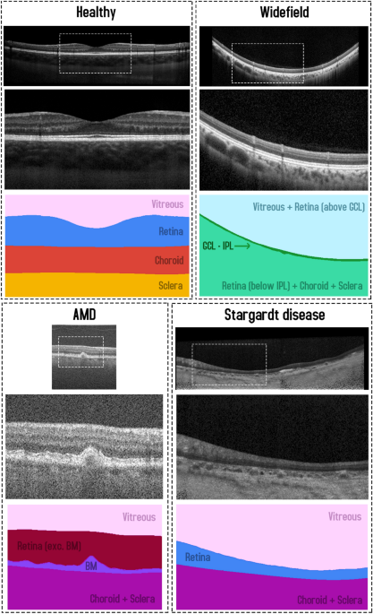
Example OCT image and corresponding semantic segmentation mask for each of the four datasets. Images are shown maintaining their aspect ratio. Each individual colour corresponds to a

different region/class as labelled. White dashed box in the topmost corresponds to the zoomed region (second and third images) for each dataset.

This dataset, described in a prior study15, consists of SD-OCT scans of patients with varying stages of Stargardt disease. Approval to identify and use SD-OCT images from patients with

genetically confirmed Stargardt disease for developing segmentation methods was obtained from the Human Ethics Office of Research Enterprise, The University of Western Australia (RA/4/1/8932

and RA/4/1/7916) and the Human Research Ethics Committee, Sir Charles Gairdner Hospital (2001-053). Scans were acquired from 18 participants, with 4 volumes (captured at different visits at

different times) of ~ 50–60 B-scans from each. The scans measure 1536 pixels wide by 496 pixels high, with a vertical scale of 3.9 µm per pixel and a horizontal scale of 5.7 µm per pixel,

this corresponds to an approximate physical area of size 8.8 × 1.9 mm (width × height). Scans were acquired using the Heidelberg Spectralis SD-OCT instrument with the ART algorithm used to

enhance the definition of each B-scan by averaging nine OCT images. Scans were taken in high-resolution mode, unless it was determined necessary to use high-speed mode owing to poor fixation

(any low-resolution scan was resized to match the resolution of the dataset). EDI was not employed. Contrast enhancement is utilised15,50 in an effort to improve layer visibility and

subsequently improve segmentation performance. After acquisition, each scan was annotated by an expert human observer, with annotations provided for two layer boundaries including: the inner

boundary of the inner limiting membrane (ILM), and the outer boundary of the retinal pigment epithelium (RPE). In some patients with Stargardt disease, the RPE and the outer retinal layers

are lost in the central region of the retina. In such cases, the remaining Bruch’s membrane (BM) that separates the residual inner retina from the choroid is marked as the outer boundary.

For each scan, a semantic segmentation mask is constructed (same pixel dimensions) with three regions: (1) vitreous (all pixels from top of image to the ILM), (2) retina (from ILM to RPE/BM)

and (3) choroid/sclera (RPE/BM to bottom of the image). An example scan and corresponding segmentation mask is provided in Fig. 1. Each participant is categorised into one of two categories

based on retinal volume (low or high). This is calculated based on the total macular retinal volume based on the boundary annotations such that there is an even number of participants in

each category. For this study, the data is divided into training (10 participants, 2426 scans), validation (2 participants, 486 scans), and testing (6 participants, 1370 scans) sets ensuring

that there is an even split of low and high volume participants in each set.

This dataset consists of OCT scans of patients exhibiting age-related macular degeneration (AMD)51. All scans were acquired using the Bioptigen SD-OCT with data sourced from four different

sites with scanning resolutions varying slightly between the sites52. No image averaging is employed. A total of 269 participants are utilised, each with a single volume of 100 scans.

However, only a subset of the scans is used. A scan is used only if it contains at least 512 pixels (approximately half the width) of available boundary annotations, otherwise it is

discarded. Each scan is then cropped to a central 512 pixels horizontally with each scan also measuring 512 pixels in height (no cropping). Each scan is supplied with boundary annotations

for three layer boundaries including the inner boundary of the ILM, the outer boundary of the retinal pigment epithelium drusen complex (RPEDC) and the outer boundary of BM. For each scan, a

semantic segmentation mask is constructed (same pixel dimensions) with four regions including: (1) vitreous (all pixels from the top of the image to the ILM), (2) retina (ILM to RPEDC), (3)

Bruch’s membrane (RPEDC to BM), and (4) choroid/sclera (BM to bottom of the image). An example scan and corresponding segmentation mask is provided in Fig. 1. A total of 163 participants

(4439 scans) are used for training, 54 participants (1481 scans) for validation, and 52 participants (1421 scans) for testing with all participants assigned randomly with no overlap or

duplication.

This dataset, which has been described in detail elsewhere53, included 12 healthy participants that had widefield OCT volume scans acquired using a widefield objective lens while maintaining

central fixation. All participants provided written consent as per protocols approved by the University of New South Wales Australia Human Research Ethics Advisory panel, and the study

adhered to the tenets of the Declaration of Helsinki. Scans were acquired using the Heidelberg Spectralis where the applied scanning protocol acquired 109 B-scans spaced 120 μm apart,

spanning a total area of 55° horizontally and 45° vertically (15.84 mm wide and 12.96 mm high), and ART was set to 16 to reduce noise. OCT B-scans were manually segmented to extract two

boundaries of interest: the inner boundary of the ganglion cell-inner layer (GCL), and the outer boundary of the inner plexiform layer (IPL). The thickness data between these two boundaries

(ganglion cell-inner plexiform layer thickness) can inform the detection and screening of a number of retinal diseases such as glaucoma54, central retinal vein occlusion55 and diabetic

macular edema56. After resizing and cropping to the region of interest, the scans measure 1392 pixels wide by 496 pixels high. For each scan, a semantic segmentation mask is constructed

(same pixel dimensions) with three regions: (1) all pixels from the top of the image to the GCL, (2) all pixels between GCL and IPL, and (3) all pixels between the IPL and the bottom of the

image. An example scan and corresponding segmentation mask is provided in Fig. 1. Scans from a total of 12 participants (~ 109 scans each, with one scan discarded from a single participant)

are utilised with 6 participants assigned for training (654 images total), 3 for validation (326 images total) and 3 for testing (327 images total). There is no overlap of participants

between the three sets.

All networks are trained to perform semantic segmentation of the OCT scans. Using a 1 × 1 convolution layer (1 × 1 strides, filter count corresponding to number of regions) followed by a

softmax activation, the output of each network consists of class probabilities corresponding to each pixel in the original input OCT image. For the Stargardt disease and widefield datasets,

the probabilities represent the classification of each pixel into one of three areas/regions of the OCT images, while there are four such areas for the healthy and AMD datasets as described

in the Data section. For each of the eight variants of the U-net architecture that are considered, we build off previous code implementations as follows: (1) baseline57, (2) dense58, (3)

attention59, (4) squeeze and excite (SE)60, (5) residual61, (6) recurrent-residual (R2)62, (7) U-Net++63, and (8) Inception64. For the comparison in this study, all networks utilise max

pooling layers (2 × 2) for down-sampling and transposed convolutions for up-sampling (2 × 2 kernel and strides). Each network consists of four pooling/up-sampling layers with 16 filters for

all convolutions in the first layer which is doubled after each pooling and subsequently halved at each up-sampling layer. Each convolution uses Glorot uniform65 kernel initialisation, and

each layer, with the exception of the output layer, is followed by batch normalisation66 and a rectified linear unit activation. We compare two variants for each architecture by considering

two and three convolutions per layer. A visual summary of each architecture is given in Fig. 2. For the residual variant, the ‘ReLU before addition’ block variant is selected while two

recurrences are performed for the R2 variant. For the SE variant, we employ the scSE module (concurrent cSE and sSE) with default ratio of 2 for the cSE component. The U-Net++ architecture

employs the same filters within the encoder and decoder (16 filters first layer, subsequently doubled in each layer) as the other architectures. However, all the intermediate layers (between

the encoder and decoder) use 16 filters each, for computational reasons.

Summary of the U-Net based architectures compared in this study. Each architecture is depicted with two pooling layers for simplicity but each uses four pooling layers in our experiments.

Arrows show direction of information flow. Coloured blocks represent particular layers as per the legend. Note: The R2, Residual and Dense variants are depicted with three convolutional

layers per block (for improved visualisation) while the others are all depicted with two (except for the Inception variant where the number of layers does not apply).

For training, the Adam optimizer67 is employed with default parameters (except for the learning rate which is set at 0.0001). A batch size of two is used and all networks are trained for 200

epochs, minimising cross-entropy as the training objective. For model selection, we use the epoch with the best Dice coefficient on the validation set. The Dice coefficient is a measure of

similarity between two samples (in this case, the predicted segmentation map and ground truth map) and is defined as:

For regularisation during training, all training samples are shuffled randomly at the beginning of each epoch. No augmentation is employed for any experiments for simplicity. The comparison

between architectures is performed by comparing the Dice coefficient on the testing set using the model selected from the best epoch. To perform a fair comparison between the network

architectures, it is necessary to run each experiment several times to ensure that there is no bias as a result of random weight initialisation and sample shuffling. Hence, all experiments

are performed three times in this study. All experiments are undertaken using Tensorflow 2.3.1 in Python 3.7.4 using an NVIDIA M40 graphics processing unit (GPU).

To statistically compare the segmentation outcomes (Dice coefficient) from the different architectures, a one-way repeated measures analysis of variance (ANOVA) was run for each of the

different datasets for both the 2 layer and 3 layer variants separately, examining the within-subject effect of network architecture. Bonferroni-adjusted pairwise comparisons were conducted

to compare between specific network architectures. An additional ANOVA was conducted to compare between the segmentation outcomes of the 2 layer and 3 layer variants.

Tables 2, 3, 4 and 5 provide a summary of the main results for the healthy dataset, Stargardt disease dataset, AMD dataset and widefield dataset, respectively. The accuracy represents the

mean (and standard deviation) overall Dice coefficient as the main performance metric, while the times (epoch training and evaluation time) together with the number of parameters allow for a

comparison of the computational complexity of the networks. Figure 3 provides a visual summary of accuracy vs. evaluation time vs. network complexity with a subplot for each of the four

datasets. It can be noted that the general clustering of the two-layer variants (squares) and three-layer variants (circles) indicates that most architectures exhibit comparable segmentation

accuracy (x-axis) with the notable exception being the R2 variant (in yellow), which showed a marginal performance improvement. Additionally, the general difference between these two

clusters (squares and circles) indicates that the three-layer variant (circles) consistently outperforms the two-layer variant (squares), but only by a small amount. While the R2 variant

(yellow) is the most accurate, it is also the slowest with respect to evaluation time (y-axis) and therefore lies in the top right corner of the subplots. However, this is not a general

trend with the Inception variant, for instance, lying in the top left corner of the subplots (slow but with relatively low accuracy compared to the other variants). Observing the subplots,

there does not appear to be any clear trends with respect to the number of network parameters (relative sizes of the circles and squares). Figures 4, 5, 6, and 7 give some example

segmentation outputs overlaid with transparency on the original OCT scans and comparisons to ground truth segmentation, demonstrating the robustness and accuracy of the segmentations for

each of the four datasets (healthy, Stargardt disease, AMD and widefield) respectively using the R2 U-Net (3 layer variant).

Segmentation accuracy (horizontal axis) vs. evaluation speed (vertical axis) vs. network parameters (size of symbol) for each of the datasets for two and three layers (square and circle

symbols respectively) for each architecture tested. Note: the axis scales on each subplot differ to support optimal visualisation.

Example segmentation outputs from the R2 U-Net (3 layer variant) for the healthy dataset overlaid on the images. Left: full image with grey dashed rectangle corresponding to the zoomed area

of the two rightmost images. Blue region: retina, red region: choroid, yellow region: sclera. Dotted lines correspond to the boundary position ground truths.

Example segmentation outputs from the R2 U-Net (3 layer variant) for the Stargardt disease dataset overlaid on the images. Left: full image with grey dashed rectangle corresponding to the

zoomed area of the two rightmost images. Blue region: retina, purple region: choroid + sclera. Dotted lines correspond to the boundary position ground truths.

Example segmentation outputs from the R2 U-Net (3 layer variant) for the AMD dataset overlaid on the images. Left: full image with grey dashed rectangle corresponding to the zoomed area of

the two rightmost images. Red region: retina (excluding BM), light purple region: BM, dark purple region: choroid + sclera. Dotted lines correspond to the boundary position ground truths.

Example segmentation outputs from the R2 U-Net (3 layer variant) for the widefield dataset overlaid on the images. Left: full image with grey dashed rectangle corresponding to the zoomed

area of the two rightmost images. Bright green region: GCL-IPL, dark green region: retina (below IPL) + choroid + sclera. Dotted lines correspond to the boundary position ground truths.

The repeated measures ANOVA revealed a significant effect of network architecture for both the healthy and Stargardt disease datasets (for both the 2 and 3 layer variants). Although the

magnitude of differences were small, the R2 architecture was found to be statistically significantly more accurate compared to some of the other architectures including the vanilla,

attention, SE and residual U-Net architectures (all p