Deep learning-enhanced light-field imaging with continuous validation

Visualizing dynamic processes over large, three-dimensional fields of view at high speed is essential for many applications in the life sciences. Light-field microscopy (LFM) has emerged as

a tool for fast volumetric image acquisition, but its effective throughput and widespread use in biology has been hampered by a computationally demanding and artifact-prone image

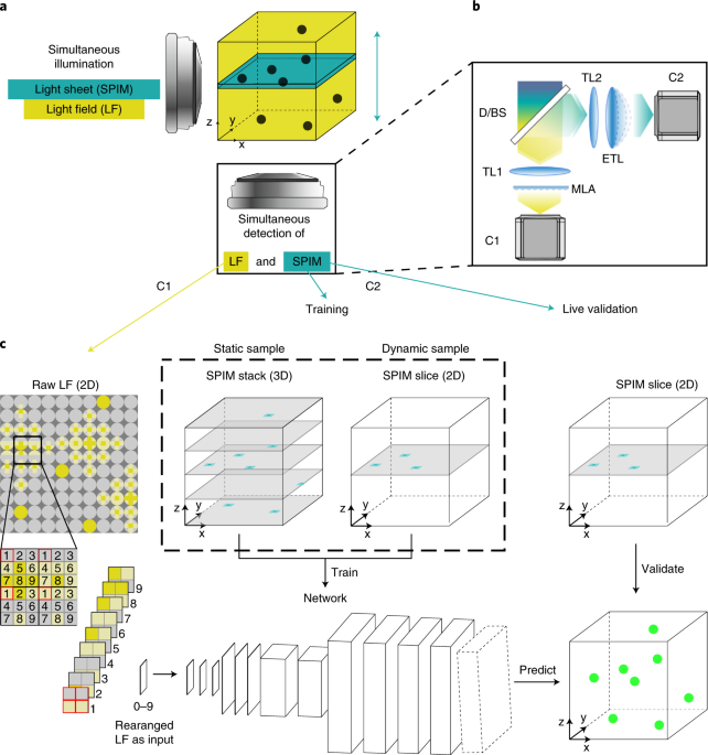
reconstruction process. Here, we present a framework for artificial intelligence–enhanced microscopy, integrating a hybrid light-field light-sheet microscope and deep learning–based volume

reconstruction. In our approach, concomitantly acquired, high-resolution two-dimensional light-sheet images continuously serve as training data and validation for the convolutional neural

network reconstructing the raw LFM data during extended volumetric time-lapse imaging experiments. Our network delivers high-quality three-dimensional reconstructions at video-rate

throughput, which can be further refined based on the high-resolution light-sheet images. We demonstrate the capabilities of our approach by imaging medaka heart dynamics and zebrafish

neural activity with volumetric imaging rates up to 100 Hz.

The datasets generated and/or analyzed during the current study are available at https://doi.org/10.5281/zenodo.4020352, https://doi.org/10.5281/zenodo.4020404 and

https://doi.org/10.5281/zenodo.4019246. Links to additional datasets are provided at https://github.com/kreshuklab/hylfm-net. Source data are provided with this paper.

The neural network code with routines for training and inference are available at https://doi.org/10.5281/zenodo.4647764.

We thank the European Molecular Biology Laboratory (EMBL) Heidelberg mechanical and electronic workshop for help as well as the IT Services Department for high-performance computing cluster

support and C. Tischer from CBA for his help with volume registration. We thank B. Balázs, Luxendo GmbH, for help with software and electronics, R. Singh and D. Kromm for general support and

C. Pape for help with benchmarking the algorithms. We also thank M. Majewsky, E. Leist and A. Saraceno for fish husbandry, and K. Slanchev and H. Baier (MPI Martinsried) as well as M.

Hoffmann and B. Judkewitz (Charite Berlin) for providing calcium reporter zebrafish lines. N.W. was supported by the Helmholtz Association under the joint research school Munich School for

Data Science (MUDS). J.G. was supported by a Research Center for Molecular Medicine (HRCMM) Career Development Fellowship, the MD/PhD program of the Medical Faculty Heidelberg, the Deutsche

Herzstiftung e.V. (S/02/17), and by an Add-On Fellowship for Interdisciplinary Science of the Joachim Herz Stiftung and is grateful to M. Gorenflo for supervision and guidance. N.N

acknowledges support from Åke Wiberg foundation, Ingabritt and Arne Lundberg foundation, and Sten K Johnson Foundation. J.C.B. acknowledges supporting fellowships from the EMBL

Interdisciplinary Postdoctoral Programme under Marie Skłodowska Curie Cofund Actions MSCACOFUND-FP (664726). L.H. thanks Luxendo GmbH for help with microscope software and equipment support.

This work was supported by the European Molecular Biology Laboratory (F.B., N.W., N.N., J.C.B., L.H., A.K. and R.P.).

Present address: Department of Informatics, Technical University of Munich, Garching, Germany

Present address: Munich School for Data Science (MUDS), Munich, Germany

These authors contributed equally: Nils Wagner, Fynn Beuttenmueller, Robert Prevedel and Anna Kreshuk.

Cell Biology and Biophysics Unit, European Molecular Biology Laboratory, Heidelberg, Germany

Nils Wagner, Fynn Beuttenmueller, Nils Norlin, Juan Carlos Boffi, Lars Hufnagel, Robert Prevedel & Anna Kreshuk

Collaboration for joint PhD degree between EMBL and Heidelberg University, Faculty of Biosciences, Heidelberg University, Heidelberg, Germany

Department of Experimental Medical Science, Lund University, Lund, Sweden

Centre for Organismal Studies, Heidelberg University, Heidelberg, Germany

Department of Pediatric Cardiology, University Hospital Heidelberg, Heidelberg, Germany

Institute of Bioengineering, School of Life Sciences, EPFL, Lausanne, Switzerland

Developmental Biology Unit, European Molecular Biology Laboratory, Heidelberg, Germany

Epigenetics and Neurobiology Unit, European Molecular Biology Laboratory, Monterotondo, Italy

Molecular Medicine Partnership Unit (MMPU), European Molecular Biology Laboratory, Heidelberg, Germany

A.K., L.H. and R.P. conceived the project. N.W. and N.N. built the imaging system and performed experiments with the help of J.G. J.G. generated transgenic animals under guidance of J.W.

F.B., A.K. and M.W. conceived the CNN architecture. F.B. and N.W. implemented the CNN and other image processing parts of the computational pipeline and evaluated its performance. J.C.B.

performed Ca2+ data analysis. A.K. and R.P. led the project and wrote the paper with input from all authors. Author order for equal contributions was determined by coin toss.

L.H. is scientific cofounder and employee of Luxendo GmbH (part of Bruker), which makes light-sheet-based microscopes commercially available, and a shareholder of Suricube GmbH, which makes

high-performance electronics and software for instrumentation control available. The other authors declare no competing interests.

Peer review information Nature Methods thanks the anonymous reviewers for their contribution to the peer review of this work. Nina Vogt was the primary editor on this article and managed its

editorial process and peer review in collaboration with the rest of the editorial team.

Publisher’s note Springer Nature remains neutral with regard to jurisdictional claims in published maps and institutional affiliations.

This architecture was used for beads and neural activity volumes. For the medaka heart, slightly different layer depth was used with the same overall structure (see Supplementary Table 1).

Res2/3d: residual blocks with 2d or 3d convolutions with kernel size (3×)3 × 3. Residual blocks contain an additional projection layer (1 × 1 or 1 × 1 × 1 convolution) if the number of input

channels is different from the number of output channels. Up2/3d: transposed convolution layers with kernel size (3×)2 × 2 and stride (1×)2 × 2. Proj2d/3d: projection layers (1 × 1 or 1 × 1

 × 1 convolutions). The numbers always correspond to the number of channels. With 19 × 19 pixel lenslets (nnum = 19) the rearranged light field input image has 192 = 361 channels. The affine

transformation layer at the end is only part of the network when training on dynamic, single plane targets; otherwise, in inference mode it might be used in post-processing to yield a SPIM

aligned prediction, or the inverse affine transformation is applied to the SPIM target for static samples to avoid unnecessary computations.

Schematic 2D drawing of the LFM-SPIM setup showing the main opto-mechanical components. The sample is illuminated through a single illumination objective with two excitation beam paths

(ocra, light sheet illumination and blue, light field selective volume illumination) combined by a dichroic mirror (D1). The fluorescence is detected by an orthogonally oriented detection

objective and optically separated onto two detection arms with a dichroic mirror (D2). Bandpass filters (BP1 and BP2) are placed in front of a tube lens (TL3,TL4) for the respective

detection path. For the light field detection path (green), the tube lens (TL4) focuses on the microlens array (ML) and the image plane (shown in magenta) displaced by one microlens focal

length is relayed by a 1-1 relay lens system (RL6) to an image plane coinciding with the camera sensor (shown in magenta). For the light sheet detection path, a combination of several relay

lenses (RL1 to RL4), a 1:1 macro lens (RL5) together with a lens pair consisting of an offset lens (OL) and an electrically tunable lens (ETL) is used to image two axially displaced

objective focal planes (shown in magenta, dotted and solid) to a common image plane at the sensor. The refocusing is achieved by applying different currents on the ETL. The mirror M1 is

placed at a Fourier plane, such that the FOV of the light sheet path can be laterally aligned to fit the light field detection FOV. For single color imaging, the dichroic mirrors D1 and D2

are replaced by beamsplitters. See Methods for details.

a, Ground truth single light sheet image. b, Subdiffraction beads reconstructed by LFM-Net and (c) iterative light field deconvolution (LFD). Scale bar is 10 µm.

Precision recall measurements (a-d) and curve (e) for HyLFM-Net-beads, LFD and LFD + CARE. In (a-d) each point represents the average for an individual axial plane. In (e) precision and

recall were averaged over all volumes, such that each point represents a threshold. All reconstructions were scaled to the SPIM ground truth to minimize L2 distance; beads were found

independently using the Difference of Gaussian (DoG) method with varying thresholds and associated with beads found in SPIM (with threshold 0.1) by Hungarian matching. N = 6716 samples were

used in each panel. Note that panel (e) is identical to Fig. 2i.

We created two kinds of samples, one with small (0.1 μm) and one with medium-sized (4 μm) beads suspended in agarose. In (a), HyLFM-Net was trained on small beads and applied to small beads.

FWHM of the beads in the reconstructed volume is shown (6025 beads measured). b, HyLFM-Net was trained on large beads and applied to large beads (682 beads measured). In (c), HyLFM-Net was

trained on small beads and used to reconstruct a volume with large beads (525 beads measured). Similarly, in (d), HyLFM-Net trained on large beads and used to reconstruct a volume with small

beads (2185 beads measured). e, SPIM image of 0.1 μm beads, (f) reconstructions of HyLFM-Net from (a), trained on small beads, (g) reconstructions from HyLFM-Net from (d), trained on large

beads. h, SPIM image of 4 μm beads, i, reconstructions of HyLFM-Net from (b), trained on large beads, (j) reconstructions of HyLFM-Net from (c), trained on small beads. Line profile is shown

to highlight a reconstruction error (red arrows), where the network reconstructs very small beads (as found in the training data) and produces an additional erroneous peak where none is

present in the ground truth SPIM volume. Shadows in (a–d) denote standard deviation. Scale bar 2 μm in (e–g), and 10 μm in (h–j).

Refinement of three differently pre-trained HyLFM networks on dynamically acquired medaka heart images. Column (a) shows SPIM ground truth plane at axial position z = -19µm. Columns (b-d)

depict corresponding slices after increasingly many refinement iterations of different pre-trained HyLFM networks. b, A statically trained HyLFM-Net (such as the one in Fig. 3b), c,

HyLFM-Net trained on LFD reconstructions of light-field images acquired on another microscope setup (Wagner, Norlin et al, Nat. Meth. 16, 497–500, 2019) and (d) HyLFM-Net trained on

medium-sized beads (see Fig. 2). e, Respective MS-SSIM image quality metrics for each network and stage of refinement. Standard deviation shown as shadows inferred from N = 756 individual

time-points. Note that depending on the domain gap, the refinement converges at different speeds, but high fidelity results can be obtained for all pre-trained networks.

a-c, Representative image plane acquired with SPIM, HyLFM-Net and LFD, respectively (standard deviation projection over time). d, Selected Ca2+-traces extracted from regions indicated in

(a-c), 36 traces with 150 time points analyzed. e, Comparison of Pearson correlation coefficients (R) of Ca2+-traces extracted by SPIM, HyLFM-Net and LFD. Note that the difference between

LFD and HyLFM-Net performance is not statistically significant (p = 0.053, Dunn-Sidak). Scale bar in (a) is 50 µm. Results representative of n = 5 individual image planes in the volume.

Volumetric HyLFM reconstruction of a beating medaka heart at 40 Hz. Volumetric reconstructions (LFD, HyLFM-Net-stat, and HyLFM-Net-stat refined) of the medaka heart at 40 Hz image

acquisition speed shown in Figs. 3 and 4. The cyan plane corresponds to the sweeping SPIM image plane. The panels from left to right show the overlay of the light sheet plane with the

respective plane from the HyLFM-Net/LFD volume, a projection of the HyLFM-Net/LFD volume rotated by 45° around the y axis, and a maximum projection of prediction/reconstruction volume along

the z, y and x axes, respectively. Scale bar 30 µm.

Supplementary Video 2 Single-plane HyLFM reconstruction of a beating medaka heart at 56 Hz. Single-plane comparison of SPIM ground truth to the corresponding plane of the prediction volume

of HyLFM-Net and reconstruction volume of LFD at indicated axial positions of the medaka heart at 56 Hz image acquisition speed (Fig. 3f,k,m). Scale bar 30 µm.

Supplementary Video 3 Single-plane HyLFM reconstruction of a beating medaka heart at 100 Hz. Single-plane comparison of SPIM ground truth to the corresponding plane of the prediction volume

of HyLFM-Net at indicated axial positions of the medaka heart at 100 Hz image acquisition speed. Scale bar 30 µm.

Supplementary Video 4 Demonstration of continuous validation and network refinement. Refinement of three differently pretrained HyLFM networks on dynamically acquired medaka heart images at

40 Hz image acquisition speed. Video of refinement experiments in Supplementary Fig. 6 (see figure caption for details).

Precision recall measurements of subdiffraction beads for HyLFM-Net-beads, LFD and LFD + CARE. Source data for Extended Data Fig. 4.

Cross-application of trained deep neural networks and the resulting FWHM of the beads in the reconstructed volume. Source data for Extended Data Fig. 5a–d.

MS-SSIM image quality metrics for each network and stage of refinement. Source data for Extended Data Fig. 6e.

Selected Ca2+ traces extracted from HyLFM, LFD and SPIM and comparison of Pearson correlation coefficients. Source data for Extended Data Fig. 7b,c.

Anyone you share the following link with will be able to read this content: