Graph pangenome captures missing heritability and empowers tomato breeding

ABSTRACT Missing heritability in genome-wide association studies defines a major problem in genetic analyses of complex biological traits1,2. The solution to this problem is to identify all

causal genetic variants and to measure their individual contributions3,4. Here we report a graph pangenome of tomato constructed by precisely cataloguing more than 19 million variants from

838 genomes, including 32 new reference-level genome assemblies. This graph pangenome was used for genome-wide association study analyses and heritability estimation of 20,323

gene-expression and metabolite traits. The average estimated trait heritability is 0.41 compared with 0.33 when using the single linear reference genome. This 24% increase in estimated

heritability is largely due to resolving incomplete linkage disequilibrium through the inclusion of additional causal structural variants identified using the graph pangenome. Moreover, by

resolving allelic and locus heterogeneity, structural variants improve the power to identify genetic factors underlying agronomically important traits leading to, for example, the

identification of two new genes potentially contributing to soluble solid content. The newly identified structural variants will facilitate genetic improvement of tomato through both

marker-assisted selection and genomic selection. Our study advances the understanding of the heritability of complex traits and demonstrates the power of the graph pangenome in crop

breeding. SIMILAR CONTENT BEING VIEWED BY OTHERS SUPER-PANGENOME ANALYSES HIGHLIGHT GENOMIC DIVERSITY AND STRUCTURAL VARIATION ACROSS WILD AND CULTIVATED TOMATO SPECIES Article Open access

06 April 2023 GWAS META-ANALYSIS USING A GRAPH-BASED PAN-GENOME ENHANCED GENE MINING EFFICIENCY FOR AGRONOMIC TRAITS IN RICE Article Open access 03 April 2025 GRAPH-BASED PAN-GENOME REVEALS

STRUCTURAL AND SEQUENCE VARIATIONS RELATED TO AGRONOMIC TRAITS AND DOMESTICATION IN CUCUMBER Article Open access 03 February 2022 MAIN Missing heritability—the discrepancy between

heritability estimates from family-based genetic studies and the variance explained by all of the significant variants in genome-wide association studies (GWAS)1,2—compromises the use of

rapidly developing genomics for understanding biological questions and crop breeding5,6,7. The resolution of missing heritability is hindered by several factors, including incomplete

detection of causal genomic variants, particularly structural variants (SVs), which leads to estimation bias caused by incomplete linkage disequilibrium (LD) between genetic markers and

causal variants, as well as genetic heterogeneity of causal variants, which reduces the statistical power of GWAS8,9,10. To overcome these bottlenecks, an exhaustive and precise catalogue of

genetic variants is required. A variation map constructed by mapping sequencing reads to a single linear reference genome generates reference bias, that is, the inability to precisely map

non-reference alleles11,12. A pangenome comprising multiple reference genomes may more fully represent species-wide genetic diversity and, as such, retains non-reference information13,14,15.

However, it is challenging to incorporate coordinates of non-reference sequences into existing analysis pipelines16. Recently, graph-based structures have been used to integrate all genetic

variants into a single genome graph, enabling thorough and accurate identification of genomic variants as well as data integration11,17,18,19. Recent studies have demonstrated the

superiority of using graph pangenomes as references in identification of SVs with short reads19,20,21,22. Here we report the construction of a variant-based graph pangenome of tomato

(_Solanum lycopersicum_), an important fruit crop and a model system for plant biology and breeding. We demonstrate its use in capturing missing heritability in GWAS, providing insights into

a classical genetics problem and facilitating genomic breeding (Extended Data Fig. 1). CONSTRUCTION OF THE GRAPH PANGENOME A high-accuracy and gapless linear reference genome is as critical

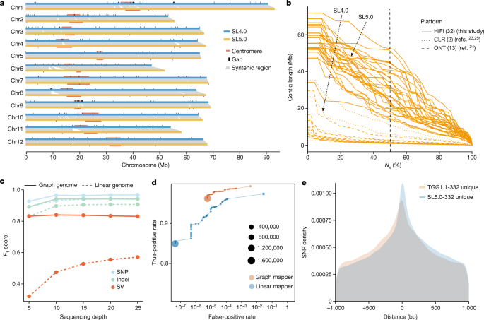
as the backbone of a graph pangenome. To this end, we assembled a state-of-the-art backbone genome (tomato cv. Heinz 1706, Build SL5.0) using high-fidelity (HiFi) long reads and

high-throughput chromosome conformation capture (Hi-C) long-range scaffolding (Extended Data Fig. 2a). The contig _N_50 size of SL5.0 is 41.7 Mb, an increase of approximately sevenfold

compared with the previous build SL4.0 (ref. 23). Moreover, SL5.0 contains 19.3 Mb more sequences than SL4.0 (801.8 Mb versus 782.5 Mb), with 43 contigs (99.8% of the assembly) ordered and

oriented on the 12 chromosomes (Fig. 1a and Extended Data Fig. 2b). Only 31 gaps remain in the SL5.0 pseudochromosomes, substantially fewer than in SL4.0 (259 gaps). Gaps remain mostly in

highly complex regions, including subtelomeres, centromeres and rDNA repeats. Both bacterial artificial chromosome clone sequences and _k_-mer analysis support the superior quality of SL5.0

(Supplementary Table 1). We performed the annotation of SL5.0 (ITAG5.0), predicting 36,648 protein-coding genes. We generated reference-level genome assemblies for another 31 accessions that

represent the diversity of the red-fruited clade of tomatoes, including 15 big-fruited tomato _S. lycopersicum_ (BIG) accessions, eight cherry tomato (_S_. _lycopersicum_ var.

_cerasiforme_, CER) accessions and eight accessions from _S_. _pimpinellifolium_ (PIM, considered to be the progenitor of cultivated tomatoes) (Supplementary Table 2 and Supplementary Fig.

1). The contig _N_50 sizes of these 31 assemblies range from 13.7 Mb to 52.2 Mb, with an average of 28.6 Mb, larger than any of the previously published tomato pangenome assemblies MAS2.0

(ref. 24) (Fig. 1b and Supplementary Table 3). We annotated repeats and predicted protein-coding genes for 45 assemblies: 31 from this study, 13 from MAS2.0 (eight BIG, three CER and two PIM

accessions)24 and 1 PIM accession from another study25. The content of repetitive sequences ranges from 60.7% to 64.0%, with an average of 62.1% (Supplementary Table 4). The number of

predicted protein-coding genes ranges from 33,863 to 37,237, with an average of 35,298 (Supplementary Table 5). The completeness of these assemblies was assessed by BUSCO analysis, which

shows an average of 96.2% single-copy Solanales genes completely assembled (Extended Data Fig. 2c). Taken together, these high-quality genome assemblies represent a robust resource to

facilitate variant detection and genomic comparison for constructing a tomato graph pangenome. With SL5.0 serving as the backbone, single-nucleotide polymorphisms (SNPs) and small insertions

and deletions (indels, 1–50 bp) identified from the 31 accessions with HiFi reads, as well as SVs (>50 bp) from all 131 accessions with long reads (a total of 100 accessions from a

previous study24 and 31 accessions from this study), were integrated into a variation graph. Complex SVs were not specifically considered when constructing the graph pangenome (Supplementary

Note 4). The resulting tomato graph pangenome (TGG1.0) spans 1,007,562,373 bp,including approximately 206 Mb absent from SL5.0. We mapped all predicted protein-coding genes to a graph

generated from all assemblies, resulting in a tomato graph annotation (TGA1.0) with 51,155 genes, of which 14,507 are from the non-reference genomes. Previous resequencing projects

accumulated 7.8 Tb of Illumina short-read data for 706 tomato accessions with a sequencing depth of greater than sixfold26,27,28,29,30,31. By mapping these short reads to TGG1.0, we

identified additional SNPs and indels that were not present in TGG1.0. After merging these variants with those from TGG1.0, we obtained a dataset comprising 17,898,731 SNPs, 1,499,161 indels

and 195,957 SVs. Integration of this updated genetic variant dataset and the SL5.0 backbone genome resulted in the generation of a new variation graph, which we designate TGG1.1. Simulation

studies indicate that the graph pangenome outperforms the linear genome at calling all types of genetic variants (SNPs, indels and SVs) (Supplementary Table 6), consistent with a recent

study on a human variation graph12,19. We compared the performance metrics for SNPs, indels and SVs derived from the graph pangenome and the linear genome. From the raw output of genotypes,

we obtained _F_1 scores (harmonic mean of precision and recall) of 0.966 for SNPs, 0.941 for indels and 0.840 for SVs in the graph pangenome using 10× sequencing data, significantly better

than those in the linear genome (0.931, 0.897 and 0.474; Wilcoxon rank sum test, _P_ = 6.30 × 10−13, _P_ = 5.04 × 10−14 and _P_ = 1.69 × 10−17, respectively) (Fig. 1c). Given that the same

variant caller DeepVariant32 was used for both datasets, higher precision and recall rate is probably driven by the higher accuracy of mapping short reads using the graph mapper (Fig. 1d).

Next, we genotyped genetic variants of 332 tomato accessions by mapping their Illumina sequences onto TGG1.1, resulting in a callset designated TGG1.1-332 that comprises 6,971,059 SNPs,

657,549 indels and 54,838 SVs. We also mapped these sequences against the linear genome SL5.0 and identified variants in a callset designated SL5.0-332 comprising 7,317,844 SNPs, 447,098

indels and 11,397 SVs. We found that SNPs that were uniquely identified by the linear reference were physically closer to their neighbouring SVs than SNPs uniquely identified by the graph

pangenome (Fig. 1e), consistent with lower levels of incorrect read mapping around SVs in the latter dataset (Extended Data Fig. 3). Furthermore, TGG1.1 contains 7,197 out of the 7,720 SNPs

(93.2%) that were verified in a DNA chip33, whereas only 6,812 (88.2%) were detected using SL5.0 as the reference. Notably, the linear genome yields only 20% of the SVs called by the graph

pangenome, indicating the high efficiency in detecting SVs using the graph pangenome. In summary, TGG1.1 represents one of the most comprehensive and accurate maps of tomato genome variation

to date. CAPTURING MISSING HERITABILITY To test the power of the graph pangenome in capturing missing heritability, we used LDAK34 to estimate the variant heritability of 20,323 molecular

traits, comprising 19,353 expression traits and 970 metabolite traits, from fruits of the 332 tomato accessions35. First, we analysed each category of genetic variants individually (that is,

only SNPs, only indels or only SVs). The average heritability estimated using the graph pangenome is higher than that using the linear reference genome for all three categories (Fig. 2a and

Supplementary Table 7). Higher SNP heritability (0.29 versus 0.28; Wilcoxon rank sum test, _P_ = 7.24 × 10−3; Extended Data Fig. 4b) is suggested despite TGG1.1-332 comprising fewer SNPs

than SL5.0-332. The results were similar when this analysis was restricted to 6,375 independent traits (square of Pearson’s correlation coefficient (_r_2) between the traits, <0.20)

(Extended Data Fig. 4a). We next analysed categories of genetic variants jointly. Estimated heritability increases with more categories in the model (Fig. 2a). When jointly analysing all

three categories of variants in a composite model, the average heritability is 0.41 in the graph pangenome callset, 24% higher than that in the linear genome callset (0.33; Wilcoxon rank sum

 test, _P_ = 1.23 × 10−217). We used the composite model to estimate the average heritability explained by SNPs, indels and SVs from TGG1.1-332, finding that SVs contribute the largest

proportion of overall heritability (0.27, 65.9%) (Extended Data Fig. 4c). Moreover, SVs contribute the largest share of heritability for approximately half of the molecular traits (10,297

out of 20,323, 50.7%) (Fig. 2b). These data indicate that the capture of missing heritability through the graph pangenome is largely due to the inclusion of more identified SVs. Incomplete

LD between molecular markers and causal variants leads to the underestimation of heritability9. SVs in close proximity to genes are probably causal variants as they could lead to

dysregulation of gene expression24,36. We observed that a large proportion of SVs are in strong LD (_R_2 > 0.7) with adjacent (50 kb on either side) SNPs and indels (61.2% and 45.5%,

respectively), but only small fractions (3.2% and 0.6%, respectively) are in complete LD (_R_2 = 1) (Fig. 2c), indicating that incomplete LD between markers and causal variants is common in

our population. Our simulation studies show that inclusion of causal variants captures some missing heritability (Supplementary Fig. 2). This could, at least partially, explain why the

average heritability increases from 0.37 to 0.41 when SVs are included in the model compared with models that consider only SNPs and indels (Fig. 2a). As an example, we studied the case of

_Solyc03G002957_, which encodes a protein that interacts with phosphoinositides. To evaluate the effects of _cis-_variants on gene expression, we partitioned genetic variants into six

categories, namely _cis_-variants (50 kb on either side of the gene) and _trans_-variants of SNPs, indels and SVs from the linear and graph pangenome callset, respectively. We found that

total heritability estimated from SL5.0-332 is 0.54 (s.d. = 0.32). By contrast, total heritability estimated from TGG1.1-332 is 0.75 (s.d. = 0.51), to which _cis-_ and _trans_-SVs jointly

contribute the largest proportions, 0.41 (s.d. = 0.34) and 0.28 (s.d. = 0.10), respectively (Fig. 2d). This indicates that SVs around this gene, most of which can be identified only using

the graph-based approach, are more likely to be causative than other variant types and contribute to the majority of total heritability. When we performed a single-variant association study,

we found that the expression of _Solyc03G002957_ is probably affected by a SV, a leading variant residing at a peak on chromosome 3 (sv3_62128422, a 2,628 bp deletion causing a truncation

at the end of the transcript) (Fig. 2e and Extended Data Figs. 5 and 6). This SV explains approximately 0.45 (s.d. = 0.63) of heritability and is present only in TGG1.1-322. However, a

significant SNP (SNP3_62204487, located about 57.6 kb upstream from the gene) exhibits modest LD with the SV (_R_2 = 0.66) (Fig. 2e) and explains 0.34 (s.d. = 0.48) of heritability in both

SL5.0-332 and TGG1.1-332. However, given the fact that SNP3_62204487 is eight genes away from the target gene, the statistical significance of this SNP could give misleading results. These

results suggest that, by addressing incomplete LD through inclusion of possibly causal SVs, the graph pangenome has the potential to capture missing heritability. A marked discrepancy still

exists between the estimated heritability and the heritability explained by GWAS significant loci2. One of the important sources is allelic heterogeneity (that is, multiple underlying

genetic variants at the same locus contribute to the same phenotype), a widespread phenomenon in complex traits that tends to impair the power of GWAS37,38. To assess the potential effect of

allelic heterogeneity on GWAS in tomato, we analysed the effects of variants in _cis-_regions (within 50 kb on either side of genes) on their corresponding gene expression (19,353 genes).

Using a single-locus mixed linear model (MLM)39 on the TGG1.1-332 callset, we detected _ci_s-expression quantitative trait loci (eQTLs) for 1,179 genes. Although the average estimated

heritability of the expression of these genes is 0.62, the average heritability explained by leading significant variants is only 0.27 (Fig. 3a). Thus, heritability contributed by nearby

genetic variants might be ‘invisible’ when considering only leading significant variants within eQTLs. When including all genetic variants in _cis_-regions of eQTLs (within 50 kb on either

side of the leading variant), the average estimated heritability increases to 0.37, therefore capturing an additional 0.10 of heritability (Fig. 3a). Moreover, there is still the expression

of 18,174 (93.9%) genes, some with large _cis_-heritability, without any significant _cis-_eQTLs (Extended Data Fig. 7a). Our study clearly suggests that allelic heterogeneity contributes to

the missing heritability of GWAS. Multilocus models have the potential to resolve allelic heterogeneity, but only small numbers of variants can be analysed simultaneously, limiting their

applications in GWAS40. Thus, to determine whether the graph pangenome enables capturing missing heritability by addressing allelic heterogeneity, we focused on associations between SVs

within gene-proximal regions (50 kb upstream and downstream) and gene expression, motivated by the assumption that SVs are likely to be causative. Using the least absolute shrinkage and

selection operator (LASSO)41, a multilocus regression model, we found that the expression of 1,787 out of the 19,353 genes is affected by at least two significantly associated SVs

(false-discovery rate = 7.53 × 10−4; permutation test). Compared with MLM, LASSO uniquely detected 1,249 _cis_-SV eQTLs, indicating its greater power in resolving allelic heterogeneity (Fig.

3b). The _cis_-heritability of the 1,249 eQTLs ranges from 0.00 to 0.59, with an average of 0.10. By contrast, we identified only 169 _cis-_SV QTLs with at least two significant SVs using

the SL5.0-332 callset, showing the need for more thorough inclusion of genetic variants to resolve allelic heterogeneity and to capture missing heritability in GWAS. Furthermore, complex SVs

such as duplications, tandem repeats and copy number variants (CNVs), most of which are probably multiallelic SVs36,42,43, could not be adequately addressed in this study. Thus, it is

probable that allelic heterogeneity may be even more prevalent than estimated here. By way of demonstration, we considered the gene _Solyc03G001472_, which encodes a protein of unknown

function. The _cis_-heritability of this gene is 0.24 (s.d. = 0.18), contributing 52% of the total heritability. There are 646 SNPs, 46 indels and three SVs within the gene-proximal region,

none of which are significantly associated with its expression when applying the MLM. Considering that the three SVs explain approximately half of the _cis_-heritability (0.12, s.d. = 0.11),

we applied the LASSO model to the three SVs, and found that two of them show significant association with gene expression, one with minor allele frequency (MAF) of 0.017 (sv3_42936717) and

the other with MAF of 0.032 (sv3_42954617) (Fig. 3c). The expression levels of different SV genotypes show that both SVs are associated with the expression of _Solyc03G001472_ (Extended Data

Fig. 7b). Overall, we show that allelic heterogeneity can be partially addressed by cataloguing of SVs exclusively identified by the graph pangenome. Locus heterogeneity—the phenomenon that

complex traits are controlled by allelic variants across multiple genes—may also decrease the statistical power of GWAS44. In theory, the LASSO model could be used to resolve locus

heterogeneity (as well as allelic heterogeneity) but, in practice, this is not feasible owing to the large number of genome-wide markers. An alternative approach is to focus on a network of

genes potentially involved in regulating specific traits. The ‘omnigenic model’ postulates that all expressed genes may be involved in the regulation of complex traits45; however, only genes

with largeeffects can be detected with a limited sample size. For gene expression, we derived a co-expression network formed by 99 modules, including 17,592 genes, using weighted

correlation network analysis (WGCNA)46 (Supplementary Table 8). Each module consists of an average of 177.7 genes, accounting for only 0.92% of the 19,353 expressed genes. Notably, we found

that variants within the proximal region of module genes on average contribute 0.22 of gene expression heritability, or 48.9% of the total estimated heritability (0.45) (Extended Data Fig.

7c). This indicates that genes in the same module, although fewer in number, may have disproportionately large effects on their corresponding module gene expression. As a consequence, to

address locus heterogeneity for complex traits, we can narrow the search space within a certain module in the co-expression network, and then focus on SVs affecting the corresponding gene

expression. To assess the effectiveness of this strategy, we concentrated on flavonoid content (comprising 38 detected metabolites35), an important tomato fruit-quality trait, with

heritability ranging from 0.07 to 1.00 (Fig. 3d and Supplementary Table 9). A co-expression network analysis shows that a module comprising 81 genes is related to the flavonoid pathway

(hereafter, the flavonoid module) (Extended Data Fig. 8). Whole-genome SVs from TGG1.1-332 contribute on average 0.21 to the heritability of the 38 metabolite contents (range, 0.00–0.58). We

found that SVs located in the proximal regions of flavonoid-module genes contribute 0.14 of heritability (Fig. 3d), suggesting that the 81 genes account for most of the genetic regulation

of flavonoid content. Using LASSO, we identified 17 out of 81 genes with _cis_-SV eQTLs (Fig. 3d and Supplementary Table 10). The 171 SVs surrounding the 17 genes (_cis-_SV set) constitute

the candidate dataset for evaluating the effect of locus heterogeneity on flavonoid content. We performed association analyses between the _cis-_SV set and the 38 metabolites using LASSO and

identified 16 SVs surrounding nine genes associated with 31 metabolites (Supplementary Table 11). Moreover, 17 out of 31 metabolites are associated with multiple genes (Fig. 3d), suggesting

that locus heterogeneity affects this complex network of flavonoids. The nine genes affecting the 31 flavonoids consist of three genes with transcription factor activity (including the

previously reported gene _SlMYB12_) and six enzyme-coding genes. In particular, Gene Ontology analysis shows that there are two transcription factors and two enzymes involved in the

flavonoid biosynthetic process (Supplementary Table 12). This is one example demonstrating how the graph pangenome-based methodology sheds new light on recovering missing heritability by

resolving locus heterogeneity. GRAPH PANGENOME EMPOWERS TOMATO BREEDING Optimal use of the extensive genome variants is expected to facilitate a paradigm shift in crop improvement47.

Significant genetic variants identified in GWAS are promising candidate markers for marker-assisted selection (MAS) in breeding. As a proof-of-concept study taking advantage of the added

value of the graph pangenome to tomato breeding, we took fruit soluble solids content (SSC), an important yield and flavour trait, as a breeding target. A previous study reported two QTLs

underlying SSC30, _Lin5_ on chromosome 9 and _SSC11.1_ on chromosome 11. To detect variants that potentially cause locus heterogeneity, we developed a universal pipeline by analysing SSC and

gene expression simultaneously using WGCNA and identified a module containing 103 genes that are probably related to SSC. SVs in the proximal regions of these genes contribute 0.33 (s.d. = 

0.21) to SSC heritability, comprising 52.9% of total heritability (0.62, s.d. = 0.68). Using LASSO, we identified _cis-_SV eQTLs in 25 genes among these module genes. Three SVs

(SV1_85728347, SV2_44168216 and SV4_54067283) in physical proximity to the corresponding genes (_Solyc01G003449_, _Solyc02G001638_ and _Solyc04G001842_) are significantly associated with SSC

(Fig. 4a). These genes are promising candidates for dissecting the genetic architecture of SSC. Moreover, the significant genetic variants identified in this study can be valuable

candidates for developing new markers to identify accessions with high SSC. We found that two of the three SVs (SV2_44168216 and SV4_54067283) significantly affect the expression of their

nearby genes (_Solyc02G001638_ and _Solyc04G001842_) (Fig. 4b). _Solyc02G001638_ encodes a PapD-like superfamily protein, and a previous study revealed that the expression of

_Solyc04G001842_ encoding a trehalose-phosphate phosphatase is negatively correlated with the contents of d-fructose and d-glucose48. Given that SV1_85728347 is not significantly associated

with the expression of _Solyc01G003449_ (Fig. 4b), we did not consider this variant for MAS. We found that selecting accessions with high SSC on the basis of favourable alleles of both

SV2_44168216 and SV4_54067283 is more efficient than selecting on the basis of only one SV (Fig. 4c). These results indicate that it is valuable to design marker assays with SVs,

highlighting the superiority of the graph pangenome for future plant breeding. Complex traits controlled by multiple small-effect loci limit the application of MAS in crop improvement.

Genomic selection provides an alternative approach that takes advantage of small-effect QTLs. Genomic selection involves the selection of elite lines on the basis of genome-estimated

breeding values from all markers, regardless of the magnitude of their effects. Using 191 metabolites of which the heritability estimated from SVs is larger than that from SNPs (0.60 versus

0.55; Wilcoxon rank sum test, _P_ = 0.032), the accuracy (_r_2 between the true phenotype and genome-estimated breeding values) of genomic selection using SVs is higher than that using SNPs

(0.11 versus 0.10; Wilcoxon rank sum test, _P_ = 3.30 × 10−32) (Fig. 4d). This demonstrates that capturing missing heritability using SVs improves the accuracy of genomic selection. We next

applied genomic selection to tomato flavour breeding. The estimated heritability of 33 flavour-related metabolites ranges from 0.21 to 1.00 (Supplementary Table 7). With the best linear

unbiased prediction, the prediction accuracy ranges from 0.00 to 0.23, 0.00 to 0.24 and 0.02 to 0.25 using SNPs, indels and SVs, respectively, and prediction accuracy using SVs is highest

for 22 of the 33 metabolites (Fig. 4e). To facilitate genomic selection in tomato breeding, we selected 20,955 candidate SVs, comprising 11,488 insertions, 9,403 deletions and 64 inversions

for the design of a DNA capture array. When applied to the genomic selection of the 33 flavour-related metabolites, the SV set exhibits only limited reduction of prediction accuracy compared

with the entire SV set (0.10 versus 0.11, Wilcoxon rank sum test, _P_ = 0.693) (Fig. 4e). As SVs can be captured by a limited number of probes (Supplementary Note), this panel potentially

provides an accurate and cost-effective platform for tomato improvement. We anticipate that future studies will validate the effectiveness of the SV array in tomato breeding. These results

also enable the advancement of SV-based genomic selection in other species. Genetic variants identified from the graph pangenome will facilitate transgenic and/or genome editing-based

breeding. To improve primer design in genome editing, we designed sgRNA primers with the protospacer adjacent motif of _Cas9_ for all predicted genes and released them in a web-based

database (http://solomics.agis.org.cn/tomato). This database also provides tools to search the comprehensive catalogue of SNPs, indels and SVs, and to design kompetitive allele-specific PCR

(KASP) markers, which can benefit the tomato research and breeding communities. DISCUSSION The state-of-the-art graph pangenome presented here incorporates genetic variants from a wide range

of tomato germplasms. The inclusion of biodiversity from non-reference accessions will serve as an important platform for next-generation genomic studies and genome-assisted breeding. In

particular, using the resources offered by the graph pangenome highlights the importance of SVs in capturing missing heritability by addressing incomplete LD, allelic heterogeneity and locus

heterogeneity. Here we used both read mapping and assembly-based methods to detect SVs and genotype SVs in a population using short reads using a graph-based method. One limitation is that

complex SVs—for example, segmental duplications, tandem repeats and CNVs—are not specifically considered in our current pipeline. Another limitation is that only SVs present in the graph

could be genotyped, and the accuracy of SV genotyping is still lower than that for SNPs and indels. Methods based on high-quality genome assemblies are superior for identifying highly

complex SVs4,49. We believe that these problems will be addressed in the future through the development of tools that can generate a unified pangenome graph and annotation graph, reinforced

by the greater availability of population-level reference-grade genome assemblies. Some statistical tools exist that consider allelic heterogeneity, although these tools often fail to detect

causal variants without high marginal _P_ values43. The power of these tools can probably be improved by incorporating SVs. Moreover, we have demonstrated the importance of locus

heterogeneity. However, we recognize that our solution to use the LASSO is suboptimal, because it is not yet computationally feasible to consider all genetic markers at once. Ideally,

multilocus tools will be developed that consider more markers. Furthermore, when it becomes feasible to genotype complex SVs, it will be necessary to develop tools that, for example, allow

for multiallelic variants, and can use these variants to capture additional missing heritability and improve the accuracy of MAS and genomic selection. METHODS TOMATO SEQUENCING AND GENOME

ASSEMBLY A total of 32 tomato accessions, including the reference cultivar Heinz 1706, were chosen from the BIG, CER and PIM groups. Genomic DNA was extracted from fresh leaves of each

accession. SMRTbell libraries were constructed according to the standard protocol of PacBio (Pacific Biosciences) and sequenced on the PacBio Sequel II platform to generate HiFi reads.

Primary assemblies were generated from three assemblers (Flye v.2.7, Hicanu v.2.0 and Hifiasm v.0.13)50,51,52 and potential misassemblies were corrected using the GALA pipeline53

(Supplementary Note). For the reference genome Heinz 1706, the Hi-C data were used to obtain a chromosome-level assembly. The remaining assemblies were anchored and oriented to chromosomes

by the reference-guided software RagTag (v.1.0.1)54 with the default parameters. GENOME ANNOTATION Protein-coding genes were predicted for each genome assembly using the MAKER2 (ref. 55) and

PRAM56 pipelines. RNA evidence was collected by aligning RNA-sequencing (RNA-seq) reads to the repeat-masked assembly using HISAT2 (v.2.10.2)57 and assembling them to transcripts with

StringTie (v.1.3.0)58. TACO (v.0.7.3)59 was applied to merge stringtie gtf (--filter-splice-juncs). Ab initio gene prediction was performed using SNAP (v.2006-07-28)60 and AUGUSTUS

(v.3.3.3)61. SNAP was trained for two rounds, and AUGUSTUS prediction was performed using the ‘tomato’ model. Proteins from SwissProt (Viridiplantae) (https://www.uniprot.org) and three

_Solanum_ species (_S. lycopersicum_ cv. Heinz 1706 ITAG4.0 (ref. 23), _Solanum pimpinellifolium_ LA2093 (ref. 25) and _Solanum tuberosum_ DM (v.6.1)62 were integrated, with redundant

sequences removed using CD-HIT (v.4.6)63 with the parameter ‘-c 0.99’. Non-redundant proteins were used for homology-based prediction using BRAKER (v.2.1.4)64 and GeneMark (v.4.3.8)65. Only

integrated gene models with AED values of <0.5 were retained. Furthermore, new gene models were predicted using PRAM. SNP AND INDEL CALLING USING HIFI READS The HiFi reads were first

mapped to SL5.0 using minimap2 (ref. 66) with the parameters ‘-a -k 19 -O 5,56 -E 4,1 -B 5 -z 400,50 -r 2k --eqx --secondary=no’. DeepVariant (v.1.0.0) with the pretrained PacBio mode

(--model_type PACBIO) was then used for variant calling of each accession, and all individual variants were merged using glnexus_cli from DeepVariant (v.0.9.0). Finally, variants that met

all of the following criteria were retained: (1) total sequencing depth from 400 to 1,500; (2) quality score ≥ 20; (3) biallelic variants; (4) length ≤ 50 bp for indels. SV DETECTION To

detect SVs using HiFi reads from the 31 accessions, we mapped HiFi reads to SL5.0 using NGLMR (v.0.2.7)67 with the default parameters. A total of four callers: Sniffles (v.1.0.12)67, SVIM

(v.1.2.0)68, CuteSV (v.1.0.10)69 and PBSV (v.2.4.0) (https://github.com/PacificBiosciences/pbsv) with the default parameters were used for variant calling in each accession. We retained

variants with a ‘pass’ flag and a read depth of at least three. Deletions ranging from 51 bp to 100 kb in length, and insertions ranging from 51 bp to 20 kb in length were retained. To

identify SVs from the 45 genome assemblies, Assemblytics70 was applied to the genome alignments generated using MUMmer (v.4.0)71 with the default parameters. For the 31 accessions with SVs

from the five callers, we merged all SVs shorter than 100 kb using SURVIVOR (v.1.0.6)8 using a maximum allowed distance of 1 kb, reporting only calls supported by at least two callers and

where the callers agreed regarding the type of variant. SVs longer than 100 kb detected by Assemblytics were retained. As the publicly available SVs from 100 tomatoes were identified using a

different version of the reference genome (SL4.0), we transformed the coordinates to SL5.0 using the LiftOver software according to the instructions provided on the UCSC website

(http://genomewiki.ucsc.edu/index.php/Minimal_Steps_For_LiftOver). CONSTRUCTION OF THE GRAPH PANGENOME SVs from the 31 accessions with HiFi reads and previously identified SVs from the 100

tomatoes were merged, and redundant SVs were removed according to instructions provided on GitHub (https://github.com/vgteam/giraffe-sv-paper/blob/master/scripts/sv). The variation graph

toolkit (vg) pipeline19 was used for the construction of TGG1.0, with SNPs and indels called from the HiFi reads. The vg pipeline was also used for variant calling with short reads. To

obtain genotypes of variants in TGG1.0, the GBWT index was created using the greedy path-cover algorithm and 32 paths, and the default minimizer length of 29 was chosen in the minimizer

index with a window size of 11. Short reads from 706 tomato accessions (>6×) were mapped to TGG1.0 with Giraffe19 and SNPs and indels were called using DeepVariant with the NGS model.

These SNPs and indels were filtered as recommended. Non-redundant SVs, SNPs and indels from both the 31 accessions with HiFi reads, the 100 accessions with ONT long reads and the 706

accessions with short reads were integrated into TGG1.1. Genotypes of SVs for the 706 accessions were called by Paragraph18 using the default parameters. GRAPH ANNOTATION To determine the

coordinates of genes from non-SL5.0 assemblies, we calculated the distance of each accession from SL5.0 using Mash (v.2.2)72. We first generated a graph format for all assemblies by

augmenting the 45 assemblies to SL5.0 using minigraph73 in increasing Mash distance with the reference SL5.0, according to the instructions provided online

(https://github.com/AnimalGenomicsETH/bovine-graphs). All of the coding sequences from the 45 accessions24,25 and the previous pangenome31 were next mapped to the graph using minigraph.

Coding sequences with more than 90% coverage and sequence identity and overlapping with the SL5.0 gene models were discarded. For genes mapped to the backbone without any protein-coding gene

annotation, we selected the longest one if annotated in more than one accession. For genes that were not mapped on the backbone of the graph, we removed redundant genes using CD-HIT with

the parameter ‘-l 0.9’ and only genes from the accession with the lowest distance from SL5.0 were retained. Finally, the gene sets mapped to the backbone and the graph were merged, and

redundant genes were removed using CD-HIT with the parameter ‘-l 0.9’. GENE EXPRESSION AND METABOLITE CONTENTS To quantify the expression of all genes, we used Kallisto (v.0.46.2)74 for all

51,155 gene models in the graph pangenome. RNA-seq data from a total of 332 accessions (217 from BIG, 98 from CER and 17 from PIM) were quantified as transcripts per million (TPM). Genes

with TPM values of >0.5 were defined as expressed. Only genes expressed in at least 100 accessions were retained for the downstream analyses. Raw expression levels were normalized with

quantile–quantile normalization. To remove potential batch effects and confounding factors affecting gene expression, the probabilistic estimation of expression residuals method75 was

applied with the top four factors as covariates. For metabolites with missing values in <100 accessions, the mean value of two replicates was used. Raw metabolite values were transformed

using the ternary logarithm and then normalized using quantile–quantile normalization. HERITABILITY ESTIMATION The LDAK-thin model76 was used to estimate the proportion of phenotypic

variance explained by genetic variants. The genetic variants were first pruned to exclude nearby SNPs in perfect LD using LDAK-thin with parameters ‘--window-prune 0.98 and --window-kb 100’.

When computing the kinship matrix, it is necessary to specify the power parameter alpha, which determines the expected relationship between per-variant heritability (_h__j_2) and MAF

(_f__j_). Specifically, it is assumed that _E_[_h__j_2] is proportional to [_f__j_(1 − _f__j_)](1 + alpha). By trying multiple values between −1 and 0, we found that alpha = −0.5 fits best

under most scenarios, indicating a tendency for per-variant heritability to decrease with lower MAF. Principal component analysis was performed using PLINK (v.2.0)77 using SNPs and indels

from TGG1.1-332, and the first four principal components were used as covariates when estimating heritability. For partitioning contributions to heritability by different types of genetic

variants, we derived the kinship for each variant category and estimated the heritability using a composite model with multiple kinship matrices. For all estimations with LDAK-thin, we added

the parameter ‘--constrain YES’ to ensure no negative estimates of heritability (if there was insufficient evidence to support the inclusion of a category, the estimated heritability was

set to zero). DEFINITION OF HERITABILITY CATEGORY We identified the coordinates of seven anchor dots that represent the seven categories as described in Supplementary Table 13. The

proportions of heritability contributed by each type of genetic variants (SNPs, indels and SVs) were used as the coordinate of each trait. Traits with heritability of zero were excluded as

we could not determine the coordinate. We next calculated the Euclidean distance between the trait and each anchor dot, and each trait was assigned to the category with the shortest

distance. GENOME-WIDE ASSOCIATION STUDY For the MLM, we used the leave-one-chromosome-out method and the mixed model implemented in GCTA39. After pruning using PLINK (v.2.0) with the

parameter ‘-indep-pairwise’ set to ‘50 5 0.2’, the pruned SNPs were used for the kinship matrix (genetic relationship matrix; GRM). For SNPs and indels, the pruned dataset (-indep-pairwise

100, 1, 0.98) was used. The first four principal components were used as covariates in the model. A Bonferroni-derived threshold (0.05/total number of markers) was used as the significance

threshold. For the LASSO model, the best linear unbiased prediction (BLUP) value estimate from LDAK (obtained from the composite model) was used as the response variable (new phenotype) for

each trait, and the significance of genetic variants was assessed using the lassopv package41. The significance threshold of LASSO was determined by 1/number of SVs and the false-discovery

rate at the threshold was estimated on the basis of permutations. QTL DEFINITION Significant variants were grouped into the same cluster if the correlation coefficient _R_2 of two adjacent

variants was >0.20 and the physical distance was <1 Mb. Clusters containing more than three significant variants were considered as candidate QTLs. For eQTL classification, _cis-_eQTLs

were inferred if the leading significant variants were <50 kb from the transcription start sites or transcription end sites of the corresponding genes; otherwise, they were considered to

be _trans-_eQTLs. CO-EXPRESSION NETWORK WGCNA46 was applied to the prefiltered expression data from 332 accessions to reconstruct gene modules exhibiting different expression patterns.

Based on the criterion of approximate scale-free topology, the number nine was chosen as the proper soft-thresholding power for a signed network. Similar expression profiles were merged to

the same module with a minimum module size set to 10 and the dissimilarity set to 0.15. GENOMIC SELECTION The rrBLUP78 package was used for genomic prediction of metabolites. SNPs and indels

with positive weight were used to calculate the kinship matrix with the A.mat function implemented in rrBLUP. The prediction accuracy was obtained by a five-fold cross-validation with five

repetitions. As the kinship matrix was calculated from genomic data, the method is also called genomic best linear unbiased prediction. REPORTING SUMMARY Further information on research

design is available in the Nature Research Reporting Summary linked to this paper. DATA AVAILABILITY All sequencing data generated in this study have been deposited at the Sequence Read

Archive (https://ncbi.nlm.nih.gov/sra) under BioProject PRJNA733299. Whole-genome sequencing data were downloaded from NCBI (BioProjects: PRJNA259308, PRJNA353161, PRJNA454805 and PRJEB5235)

and RNA-seq data were downloaded from the NCBI (BioProject: PRJNA396272). All assemblies with annotations, variant VCF files and graph files are available at the SolOmics database

(http://solomics.agis.org.cn/tomato/ftp) and Sol Genomics Network (https://solgenomics.net/ftp/genomes/TGG/). The InterPro database was downloaded from https://www.ebi.ac.uk/interpro/. The

UniProtKB/SwissProt database is available online (https://www.uniprot.org). Source data are provided with this paper. CODE AVAILABILITY All code associated with this project is available at

GitHub (https://github.com/YaoZhou89/TGG). REFERENCES * Maher, B. Personal genomes: the case of the missing heritability. _Nature_ 456, 18–21 (2008). Article  CAS  PubMed  Google Scholar  *

Manolio, T. A. et al. Finding the missing heritability of complex diseases. _Nature_ 461, 747–753 (2009). Article  ADS  CAS  PubMed  PubMed Central  Google Scholar  * Young, A. I. Solving

the missing heritability problem. _PLoS Genet._ 15, e1008222 (2019). Article  CAS  PubMed  PubMed Central  Google Scholar  * De Coster, W., Weissensteiner, M. H. & Sedlazeck, F. J.

Towards population-scale long-read sequencing. _Nat. Rev. Genet._ 22, 572–587 (2021). Article  PubMed  PubMed Central  CAS  Google Scholar  * Visscher, P. M. Sizing up human height

variation. _Nat. Genet._ 40, 489–490 (2008). Article  CAS  PubMed  Google Scholar  * Hemani, G., Knott, S. & Haley, C. An evolutionary perspective on epistasis and the missing

heritability. _PLoS Genet._ 9, e1003295 (2013). Article  CAS  PubMed  PubMed Central  Google Scholar  * Brachi, B., Morris, G. P. & Borevitz, J. O. Genome-wide association studies in

plants: the missing heritability is in the field. _Genome Biol._ 12, 232 (2011). Article  PubMed  PubMed Central  Google Scholar  * Jeffares, D. C. et al. Transient structural variations

have strong effects on quantitative traits and reproductive isolation in fission yeast. _Nat. Commun._ 8, 14061 (2017). Article  ADS  CAS  PubMed  PubMed Central  Google Scholar  * Yang, J.

et al. Common SNPs explain a large proportion of the heritability for human height. _Nat. Genet._ 42, 565–569 (2010). Article  CAS  PubMed  PubMed Central  Google Scholar  * Eichler, E. E.

et al. Missing heritability and strategies for finding the underlying causes of complex disease. _Nat. Rev. Genet._ 11, 446–450 (2010). Article  CAS  PubMed  PubMed Central  Google Scholar 

* Garrison, E. et al. Variation graph toolkit improves read mapping by representing genetic variation in the reference. _Nat. Biotechnol._ 36, 875–879 (2018). Article  CAS  PubMed  PubMed

Central  Google Scholar  * Martiniano, R., Garrison, E., Jones, E. R., Manica, A. & Durbin, R. Removing reference bias and improving indel calling in ancient DNA data analysis by mapping

to a sequence variation graph. _Genome Biol._ 21, 250 (2020). Article  CAS  PubMed  PubMed Central  Google Scholar  * The 1000 Genomes Project Consortium. A global reference for human

genetic variation. _Nature_ 526, 68–74 (2015). Article  CAS  Google Scholar  * Jayakodi, M. et al. The barley pan-genome reveals the hidden legacy of mutation breeding. _Nature_ 588, 284–289

(2020). Article  ADS  CAS  PubMed  PubMed Central  Google Scholar  * Hufford, M. B. et al. De novo assembly, annotation, and comparative analysis of 26 diverse maize genomes. _Science_ 373,

655–662 (2021). Article  ADS  CAS  PubMed  PubMed Central  Google Scholar  * The Computational Pan-Genomics Consortium. Computational pan-genomics: status, promises and challenges. _Brief.

Bioinform._ 19, 118–135 (2018). Google Scholar  * Rakocevic, G. et al. Fast and accurate genomic analyses using genome graphs. _Nat. Genet._ 51, 354–362 (2019). Article  CAS  PubMed  Google

Scholar  * Chen, S. et al. Paragraph: a graph-based structural variant genotyper for short-read sequence data. _Genome Biol._ 20, 291 (2019). Article  PubMed  PubMed Central  Google Scholar

  * Sirén, J. et al. Pangenomics enables genotyping of known structural variants in 5202 diverse genomes. _Science_ 374, eabg8871 (2021). Article  CAS  Google Scholar  * Liu, Y. et al.

Pan-genome of wild and cultivated soybeans. _Cell_ 182, 162–176 (2020). Article  CAS  PubMed  Google Scholar  * Qin, P. et al. Pan-genome analysis of 33 genetically diverse rice accessions

reveals hidden genomic variations. _Cell_ 184, 3542–3558 (2021). Article  CAS  PubMed  Google Scholar  * Ebert, P. et al. Haplotype-resolved diverse human genomes and integrated analysis of

structural variation. _Science_ 372, eabf7117 (2021). Article  CAS  PubMed  PubMed Central  Google Scholar  * Hosmani, P. S. et al. An improved de novo assembly and annotation of the tomato

reference genome using single-molecule sequencing, Hi-C proximity ligation and optical maps. Preprint at _bioRxiv_ https://doi.org/10.1101/767764 (2019). * Alonge, M. et al. Major impacts of

widespread structural variation on gene expression and crop improvement in tomato. _Cell_ 182, 145–161 (2020). Article  CAS  PubMed  PubMed Central  Google Scholar  * Wang, X. et al. Genome

of _Solanum pimpinellifolium_ provides insights into structural variants during tomato breeding. _Nat. Commun._ 11, 5817 (2020). Article  ADS  CAS  PubMed  PubMed Central  Google Scholar  *

Causse, M. et al. Whole genome resequencing in tomato reveals variation associated with introgression and breeding events. _BMC Genom._ 14, 791 (2013). Article  CAS  Google Scholar  *

Aflitos, S. et al. Exploring genetic variation in the tomato (_Solanum_ section _Lycopersicon_) clade by whole‐genome sequencing. _Plant J._ 80, 136–148 (2014). Article  PubMed  CAS  Google

Scholar  * Bolger, A. et al. The genome of the stress-tolerant wild tomato species _Solanum pennellii_. _Nat. Genet._ 46, 1034–1038 (2014). Article  CAS  PubMed  PubMed Central  Google

Scholar  * Lin, T. et al. Genomic analyses provide insights into the history of tomato breeding. _Nat. Genet._ 46, 1220–1226 (2014). Article  CAS  PubMed  Google Scholar  * Tieman, D. et al.

A chemical genetic roadmap to improved tomato flavor. _Science_ 355, 391–394 (2017). Article  ADS  CAS  PubMed  Google Scholar  * Gao, L. et al. The tomato pan-genome uncovers new genes and

a rare allele regulating fruit flavor. _Nat. Genet._ 51, 1044–1051 (2019). Article  CAS  PubMed  Google Scholar  * Poplin, R. et al. A universal SNP and small-indel variant caller using

deep neural networks. _Nat. Biotechnol._ 36, 983–987 (2018). Article  CAS  PubMed  Google Scholar  * Sim, S.-C. et al. Development of a large SNP genotyping array and generation of

high-density genetic maps in tomato. _PLoS ONE_ 7, e40563 (2012). Article  ADS  CAS  PubMed  PubMed Central  Google Scholar  * Speed, D., Hemani, G., Johnson, M. R. & Balding, D. J.

Improved heritability estimation from genome-wide SNPs. _Am. J. Hum. Genet._ 91, 1011–1021 (2012). Article  CAS  PubMed  PubMed Central  Google Scholar  * Zhu, G. et al. Rewiring of the

fruit metabolome in tomato breeding. _Cell_ 172, 249–261 (2018). Article  CAS  PubMed  Google Scholar  * Vinces, M. D., Legendre, M., Caldara, M., Hagihara, M. & Verstrepen, K. J.

Unstable tandem repeats in promoters confer transcriptional evolvability. _Science_ 324, 1213–1216 (2009). Article  ADS  CAS  PubMed  PubMed Central  Google Scholar  * The GTEx Consortium.

The GTEx Consortium atlas of genetic regulatory effects across human tissues. _Science_ 369, 1318–1330 (2020). Article  PubMed Central  CAS  Google Scholar  * Hormozdiari, F. et al.

Widespread allelic heterogeneity in complex traits. _Am. J. Hum. Genet._ 100, 789–802 (2017). Article  CAS  PubMed  PubMed Central  Google Scholar  * Yang, J., Lee, S. H., Goddard, M. E.

& Visscher, P. M. GCTA: a tool for genome-wide complex trait analysis. _Am. J. Hum. Genet._ 88, 76–82 (2011). Article  CAS  PubMed  PubMed Central  Google Scholar  * Hormozdiari, F.,

Jung, J., Eskin, E. & Joo, J. W. J. MARS: leveraging allelic heterogeneity to increase power of association testing. _Genome Biol._ 22, 128 (2021). Article  CAS  PubMed  PubMed Central 

Google Scholar  * Wang, L. & Michoel, T. Controlling false discoveries in Bayesian gene networks with lasso regression _p_-values. Preprint at _arXiv_ https://arxiv.org/abs/1701.07011

(2017). * Sudmant, P. H. et al. An integrated map of structural variation in 2,504 human genomes. _Nature_ 526, 75–81 (2015). Article  CAS  PubMed  PubMed Central  Google Scholar  * Collins,

R. L. et al. A structural variation reference for medical and population genetics. _Nature_ 581, 444–451 (2020). Article  ADS  CAS  PubMed  PubMed Central  Google Scholar  * Mancuso, N. et

al. Probabilistic fine-mapping of transcriptome-wide association studies. _Nat. Genet._ 51, 675–682 (2019). Article  CAS  PubMed  PubMed Central  Google Scholar  * Boyle, E. A., Li, Y. I.

& Pritchard, J. K. An expanded view of complex traits: from polygenic to omnigenic. _Cell_ 169, 1177–1186 (2017). Article  CAS  PubMed  PubMed Central  Google Scholar  * Langfelder, P.

& Horvath, S. WGCNA: an R package for weighted correlation network analysis. _BMC Bioinform._ 9, 559 (2008). Article  CAS  Google Scholar  * Della Coletta, R., Qiu, Y., Ou, S., Hufford,

M. B. & Hirsch, C. N. How the pan-genome is changing crop genomics and improvement. _Genome Biol._ 22, 3 (2021). Article  PubMed  PubMed Central  Google Scholar  * Li, N. et al.

Identification of the carbohydrate and organic acid metabolism genes responsible for brix in tomato fruit by transcriptome and metabolome analysis. _Front. Genet._ 12, 714942 (2021). Article

  CAS  PubMed  PubMed Central  Google Scholar  * Mahmoud, M. et al. Structural variant calling: the long and the short of it. _Genome Biol._ 20, 246 (2019). Article  PubMed  PubMed Central 

Google Scholar  * Kolmogorov, M., Yuan, J., Lin, Y. & Pevzner, P. A. Assembly of long, error-prone reads using repeat graphs. _Nat. Biotechnol._ 37, 540–546 (2019). Article  CAS  PubMed

  Google Scholar  * Nurk, S. et al. HiCanu: accurate assembly of segmental duplications, satellites, and allelic variants from high-fidelity long reads. _Genome Res._ 30, 1291–1305 (2020).

Article  CAS  PubMed  PubMed Central  Google Scholar  * Cheng, H., Concepcion, G. T., Feng, X., Zhang, H. & Li, H. Haplotype-resolved de novo assembly using phased assembly graphs with

hifiasm. _Nat. Methods_ 18, 170–175 (2021). Article  CAS  PubMed  PubMed Central  Google Scholar  * Awad, M. & Gan, X. GALA: gap-free chromosome-scale assembly with long reads. Preprint

at _bioRxiv_ https://doi.org/10.1101/2020.05.15.097428 (2020). * Alonge, M. et al. RaGOO: fast and accurate reference-guided scaffolding of draft genomes. _Genome Biol._ 20, 224 (2019).

Article  PubMed  PubMed Central  Google Scholar  * Holt, C. & Yandell, M. MAKER2: an annotation pipeline and genome-database management tool for second-generation genome projects. _BMC

Bioinform._ 12, 491 (2011). Article  Google Scholar  * Liu, P., Soukup, A. A., Bresnick, E. H., Dewey, C. N. & Keleş, S. PRAM: a novel pooling approach for discovering intergenic

transcripts from large-scale RNA sequencing experiments. _Genome Res._ 30, 1655–1666 (2020). Article  CAS  PubMed  PubMed Central  Google Scholar  * Kim, D., Paggi, J. M., Park, C., Bennett,

C. & Salzberg, S. L. Graph-based genome alignment and genotyping with HISAT2 and HISAT-genotype. _Nat. Biotechnol._ 37, 907–915 (2019). Article  CAS  PubMed  PubMed Central  Google

Scholar  * Pertea, M. et al. StringTie enables improved reconstruction of a transcriptome from RNA-seq reads. _Nat. Biotechnol._ 33, 290–295 (2015). Article  CAS  PubMed  PubMed Central 

Google Scholar  * Niknafs, Y. S., Pandian, B., Iyer, H. K., Chinnaiyan, A. M. & Iyer, M. K. TACO produces robust multisample transcriptome assemblies from RNA-seq. _Nat. Methods_ 14,

68–70 (2017). Article  CAS  PubMed  Google Scholar  * Korf, I. Gene finding in novel genomes. _BMC Bioinform._ 5, 59 (2004). Article  Google Scholar  * Stanke, M. et al. AUGUSTUS: ab initio

prediction of alternative transcripts. _Nucleic Acids Res._ 34, W435–W439 (2006). Article  CAS  PubMed  PubMed Central  Google Scholar  * Pham, G. M. et al. Construction of a

chromosome-scale long-read reference genome assembly for potato. _Gigascience_ 9, giaa100 (2020). Article  PubMed  PubMed Central  CAS  Google Scholar  * Fu, L., Niu, B., Zhu, Z., Wu, S.

& Li, W. CD-HIT: accelerated for clustering the next-generation sequencing data. _Bioinformatics_ 28, 3150–3152 (2012). Article  CAS  PubMed  PubMed Central  Google Scholar  * Hoff, K.,

Lomsadze, A., Borodovsky, M. & Stanke, M. Whole-genome annotation with BRAKER. _Methods Mol. Biol._ 1962, 65–95 (2019). Article  CAS  PubMed  PubMed Central  Google Scholar  * Brůna, T.,

Lomsadze, A. & Borodovsky, M. GeneMark-EP+: eukaryotic gene prediction with self-training in the space of genes and proteins. _NAR Genom. Bioinform._ 2, lqaa026 (2020). Article  PubMed

  PubMed Central  CAS  Google Scholar  * Li, H. Minimap2: pairwise alignment for nucleotide sequences. _Bioinformatics_ 34, 3094–3100 (2018). Article  CAS  PubMed  PubMed Central  Google

Scholar  * Sedlazeck, F. J. et al. Accurate detection of complex structural variations using single-molecule sequencing. _Nat. Methods_ 15, 461–468 (2018). Article  CAS  PubMed  PubMed

Central  Google Scholar  * Heller, D. & Vingron, M. SVIM: structural variant identification using mapped long reads. _Bioinformatics_ 35, 2907–2915 (2019). Article  CAS  PubMed  PubMed

Central  Google Scholar  * Jiang, T. et al. Long-read-based human genomic structural variation detection with cuteSV. _Genome Biol._ 21, 189 (2020). Article  CAS  PubMed  PubMed Central 

Google Scholar  * Nattestad, M. & Schatz, M. C. Assemblytics: a web analytics tool for the detection of variants from an assembly. _Bioinformatics_ 32, 3021–3023 (2016). Article  CAS 

PubMed  PubMed Central  Google Scholar  * Marçais, G. et al. MUMmer4: a fast and versatile genome alignment system. _PLoS Comput. Biol._ 14, e1005944 (2018). Article  PubMed  PubMed Central

  CAS  Google Scholar  * Ondov, B. D. et al. Mash: fast genome and metagenome distance estimation using MinHash. _Genome Biol._ 17, 132 (2016). Article  PubMed  PubMed Central  CAS  Google

Scholar  * Li, H., Feng, X. & Chu, C. The design and construction of reference pangenome graphs with minigraph. _Genome Biol._ 21, 265 (2020). Article  PubMed  PubMed Central  Google

Scholar  * Bray, N. L., Pimentel, H., Melsted, P. & Pachter, L. Near-optimal probabilistic RNA-seq quantification. _Nat. Biotechnol._ 34, 525–527 (2016). Article  CAS  PubMed  Google

Scholar  * Stegle, O., Parts, L., Piipari, M., Winn, J. & Durbin, R. Using probabilistic estimation of expression residuals (PEER) to obtain increased power and interpretability of gene

expression analyses. _Nat. Protoc._ 7, 500–507 (2012). Article  CAS  PubMed  PubMed Central  Google Scholar  * Speed, D., Holmes, J. & Balding, D. J. Evaluating and improving

heritability models using summary statistics. _Nat. Genet._ 52, 458–462 (2020). Article  CAS  PubMed  Google Scholar  * Purcell, S. et al. PLINK: a tool set for whole-genome association and

population-based linkage analyses. _Am. J. Hum. Genet._ 81, 559–575 (2007). Article  CAS  PubMed  PubMed Central  Google Scholar  * Endelman, J. B. Ridge regression and other kernels for

genomic selection with R package rrBLUP. _Plant Genome_ 4, 250–255 (2011). Article  Google Scholar  * Kearse, M. et al. Geneious Basic: an integrated and extendable desktop software platform

for the organization and analysis of sequence data. _Bioinformatics_ 28, 1647–1649 (2012). Article  PubMed  PubMed Central  Google Scholar  Download references ACKNOWLEDGEMENTS We thank N.

Stein, M. Mascher and J. Giovannoni for comments and advice; G. Zhu for providing metabolite data; and Q. Zhang for suggestions on the estimation of heritability. This work was supported by

grants from the National Natural Science Foundation of China (no. 31991180 to S.H. and no. 31801441 to Y. Zhou), the National Key Research and Development Program of China (no.

2019YFA0906200 to S.H.), the Key Research and Development Program of Guangdong Province (no. 2021B0707010005 to J.Z.), the Shenzhen Science and Technology Program (no. KQTD2016113010482651

to S.H.), the Agricultural Science and Technology Innovation Program (CAAS-ZDRW202103 to S.H.) and the US National Science Foundation (IOS-1855585 to Z.F.). AUTHOR INFORMATION Author notes *

These authors contributed equally: Yao Zhou, Zhiyang Zhang, Zhigui Bao AUTHORS AND AFFILIATIONS * Shenzhen Branch, Guangdong Laboratory of Lingnan Modern Agriculture, Genome Analysis

Laboratory of the Ministry of Agriculture and Rural Affairs, Agricultural Genomics Institute at Shenzhen, Chinese Academy of Agricultural Sciences, Shenzhen, China Yao Zhou, Zhiyang Zhang, 

Zhigui Bao, Hongbo Li, Yaqing Lyu, Yanjun Zan, Yaoyao Wu, Lin Cheng, Yuhan Fang, Kun Wu, Hongjun Lyu & Sanwen Huang * Umeå Plant Science Center, Department of Forestry Genetics and Plant

Physiology, Swedish University of Agricultural Sciences, Umeå, Sweden Yanjun Zan * Key Laboratory of Biology and Genetic Improvement of Horticultural Crops of the Ministry of Agriculture,

Sino-Dutch Joint Laboratory of Horticultural Genomics, and Institute of Vegetables and Flowers, Chinese Academy of Agricultural Sciences, Beijing, China Jinzhe Zhang * Institute of

Vegetables, Shandong Academy of Agricultural Sciences, Shandong Province Key Laboratory for Biology of Greenhouse Vegetables, Shandong Branch of National Improvement Center for Vegetables,

Huang-Huai-Hai Region Scientific Observation and Experimental Station of Vegetables, Ministry of Agriculture and Rural Affairs, Jinan, China Hongjun Lyu * State Key Laboratory of

Agrobiotechnology, College of Horticulture, China Agricultural University, Beijing, China Tao Lin * Boke Biotech, Wuxi, China Qiang Gao * Boyce Thompson Institute, Cornell University,

Ithaca, NY, USA Surya Saha, Lukas Mueller & Zhangjun Fei * Robert W. Holley Center for Agriculture and Health, US Department of Agriculture, Agricultural Research Service, Ithaca, NY,

USA Zhangjun Fei * Institute of Integrative Biology & Zurich, Basel Plant Science Center, ETH Zurich, Zurich, Switzerland Thomas Städler * Department of Botany and Plant Sciences,

University of California, Riverside, CA, USA Shizhong Xu * Department of Crop and Soil Sciences, Washington State University, Pullman, WA, USA Zhiwu Zhang * Quantitative Genetics and

Genomics (QGG), Aarhus University, Aarhus, Denmark Doug Speed Authors * Yao Zhou View author publications You can also search for this author inPubMed Google Scholar * Zhiyang Zhang View

author publications You can also search for this author inPubMed Google Scholar * Zhigui Bao View author publications You can also search for this author inPubMed Google Scholar * Hongbo Li

View author publications You can also search for this author inPubMed Google Scholar * Yaqing Lyu View author publications You can also search for this author inPubMed Google Scholar *

Yanjun Zan View author publications You can also search for this author inPubMed Google Scholar * Yaoyao Wu View author publications You can also search for this author inPubMed Google

Scholar * Lin Cheng View author publications You can also search for this author inPubMed Google Scholar * Yuhan Fang View author publications You can also search for this author inPubMed 

Google Scholar * Kun Wu View author publications You can also search for this author inPubMed Google Scholar * Jinzhe Zhang View author publications You can also search for this author

inPubMed Google Scholar * Hongjun Lyu View author publications You can also search for this author inPubMed Google Scholar * Tao Lin View author publications You can also search for this

author inPubMed Google Scholar * Qiang Gao View author publications You can also search for this author inPubMed Google Scholar * Surya Saha View author publications You can also search for

this author inPubMed Google Scholar * Lukas Mueller View author publications You can also search for this author inPubMed Google Scholar * Zhangjun Fei View author publications You can also

search for this author inPubMed Google Scholar * Thomas Städler View author publications You can also search for this author inPubMed Google Scholar * Shizhong Xu View author publications

You can also search for this author inPubMed Google Scholar * Zhiwu Zhang View author publications You can also search for this author inPubMed Google Scholar * Doug Speed View author

publications You can also search for this author inPubMed Google Scholar * Sanwen Huang View author publications You can also search for this author inPubMed Google Scholar CONTRIBUTIONS

S.H. and Y. Zhou conceived and designed the research. Y. Zhou, J.Z., Y.L., H. Lyu and Y.W. participated in the material preparation. S.S. and L.M. provided the Hi-C data of Heinz 1706. Y.

Zhou, Z.B. and T.L. contributed to genome assembly. Z.B. contributed to genome annotation. Y. Zhou, Zhiyang Zhang and L.C. detected genetic variants. Y. Zhou and Z.B. constructed graph

pangenome and annotation. Y. Zhou and Zhiyang Zhang performed gene expression and metabolites analysis. Y. Zhou, Z.B., Zhiwu Zhang, S.X. and D.S. contributed to heritability estimation and

genome-wide association study. Zhiyang Zhang contributed to co-expression network analysis. Y. Zhou and Z.B. contributed to breeding analysis. Y. Zhou and Q.G. designed the SV panel of DNA

capture array. K.W. and Y.W. provided metabolites and QTL data. H. Li and Y.F. contributed to computational analysis. Y. Zan, Z.F. and T.S contributed to statistical analysis. D.S., T.S.,

Z.F., Zhiwu Zhang, S.X., Y. Zan, Y.F. and H. Li revised the manuscript. S.H., Y. Zhou and Zhiyang Zhang wrote the manuscript. S.H. supervised the research. All of the authors read, edited

and approved the manuscript. CORRESPONDING AUTHOR Correspondence to Sanwen Huang. ETHICS DECLARATIONS COMPETING INTERESTS The authors declare no competing interests. PEER REVIEW PEER REVIEW

INFORMATION _Nature_ thanks Mathilde Causse, Erik Garrison and the other, anonymous, reviewer(s) for their contribution to the peer review of this work. Peer reviewer reports are available.

ADDITIONAL INFORMATION PUBLISHER’S NOTE Springer Nature remains neutral with regard to jurisdictional claims in published maps and institutional affiliations. EXTENDED DATA FIGURES AND

TABLES EXTENDED DATA FIG. 1 LAYOUT OF THE TOMATO GRAPH PANGENOME STUDY. A) Data used for constructing the tomato graph pangenome. B) Sketch of the tomato graph pangenome. C) Profiles of

metabolome and transcriptome. D–F) Potential sources of missing heritability: incomplete linkage disequilibrium (D), allelic heterogeneity underlying gene expression (E), and locus

heterogeneity represented in a co-expression network (F). Genes affecting the different steps of the same pathway might have the same effect on the final product. Yellow stars represent

causal mutations. G) Practical application of genomic breeding such as genomic selection (GS), marker-assisted selection (MAS) and transgenic/gene editing. EXTENDED DATA FIG. 2

CHARACTERISTICS OF TOMATO GENOME ASSEMBLIES. A) Hi-C heatmap of SL5.0. Darker red indicates higher contact probability. B) Structural variants between builds SL4.0 (blue) and SL5.0 (yellow).

Insertions, deletions, duplications and inversions between SL4.0 and SL5.0 are labelled with unique colour for each type of variants. C) Benchmarking Universal Single-Copy Orthologs (BUSCO)

evaluation for the tomato genome assemblies. EXTENDED DATA FIG. 3 READ ALIGNMENTS TO THE GRAPH PANGENOME AND THE LINEAR GENOME. Visualization of alignments of the same reads in a region by

Geneious software79 to compare differences between the graph mapper (Giraffe) (A) and the linear mapper (bwa) (B). An 81-bp deletion can be detected accurately in the graph pangenome, but

soft-clipped sequences are detected in the linear genome with five false-positive SNPs (indicated by red stars). EXTENDED DATA FIG. 4 EVALUATION OF CONTRIBUTIONS TO HERITABILITY BY DIFFERENT

VARIANT TYPES. A) Comparison of heritability estimated from different combinations of genetic variants from SL5.0-332 and TGG1.1-332. B) Comparison of estimated heritability based on SNPs

of different groups. n = 6,375 independent traits (A, B) were evaluated. ‘Overlapping’ refers to SNPs found in both TGG1.1-332 and SL5.0-332. ‘Unique’ refers to SNPs uniquely identified in

either TGG1.1-332 or SL5.0-332. Box and whisker plots (A, B) with centre line = median, cross = mean, box limits = upper and lower quartiles, whiskers = 1.5 × interquartile range and solid

points = outliers. C) Heritability contributed by different variant categories using a composite model. Source data EXTENDED DATA FIG. 5 GENE STRUCTURE OF _SOLYC03G002957_. A) Different gene

structures of _Solyc03G002957_; gene structures from three assemblies (TS12, SL5.0, and PP) are represented. The 2,628-bp deletion occurs at the end of the transcript. The 8,681-bp deletion

in the LTR region results in a different annotation at the 3’ end of the transcript. B) Graph representation of adjacent regions of _Solyc03G002957_. The graph was generated from the 46

assemblies shown in c). C) Linear representation of regions adjacent to _Solyc03G002957_. Multiple alignment of all assemblies was performed using pggb (https://github.com/pangenome/pggb).

The 8,681-bp deletion in the LTR region exists in all assemblies harbouring the haplotype with the 2,628-bp deletion. Furthermore, the multiallelic LTR deletion is represented in TGG1.1 but

was filtered out in TGG1.1-332 due to low frequency, implying the potential for further improvements in genotyping multiallelic SVs using short reads. EXTENDED DATA FIG. 6 INTEGRATED GENOME

VIEWER OF GENE MODELS ACCORDING TO SL5.0 AND SL4.0. This gene was misannotated as two separate genes in ITAG 4.0, possibly due to an LTR/_Gypsy_ retrotransposon (12,295 bp) at the sixth

intron. Blue and green lines with mRNA IDs shown represent the complete gene structure. UTRs are illustrated by thin bars, ORFs by thick bars and introns by thin lines. Arrowheads within the

bars indicate transcriptional orientation. RNA-seq reads mapped to _Solyc03G002957_ in SL5.0 are shown in the lower part of this figure. EXTENDED DATA FIG. 7 ALLELIC AND LOCUS HETEROGENEITY

IN GWAS. A) Comparison of heritability estimated from leading significant variants (if present) and all genetic variants in the _cis_ regions (within 50 kb upstream and downstream of a

gene) for all expressed genes. If no significant variants are detected, \({h}_{{cis\; gwas}}^{2}\) is zero. B) Box plots of best linear unbiased prediction (BLUP) for the expression of

_Solyc03G001472_ in different genotypes of the two significant SVs. n represents number of accessions of each group. The total sample size is 331 (only groups with at least three accessions

were analysed). The _P_-value was calculated from Kruskal-Wallis rank sum test. Box and whisker plots with centre line = median, cross = mean, box limits = upper and lower quartiles,

whiskers = 1.5 × interquartile range and solid points = outliers. C) Heritability of gene expression contributed by different types of variants (SNPs, indels and SVs) within module and

non-module genes in a composite model. Source data EXTENDED DATA FIG. 8 CO-EXPRESSION NETWORK OF EXPRESSED GENES. The hub genes of each module (a total of 99) are visually magnified and

coloured in black and non-hub genes are coloured in grey. The soluble solids content (SSC) and flavonoid module genes are coloured in blue and red, respectively. There are 5,520 expressed

genes in the network with 190,606 links (threshold > 0.05). SUPPLEMENTARY INFORMATION SUPPLEMENTARY INFORMATION Supplementary Methods and Results are provided within Supplementary Notes

1–9 and Supplementary Figs. 1–20. REPORTING SUMMARY PEER REVIEW FILE SUPPLEMENTARY TABLES 1–16. SOURCE DATA SOURCE DATA FIG. 1 SOURCE DATA FIG. 2 SOURCE DATA FIG. 3 SOURCE DATA FIG. 4 SOURCE

DATA EXTENDED DATA FIG. 4 SOURCE DATA EXTENDED DATA FIG. 7 RIGHTS AND PERMISSIONS OPEN ACCESS This article is licensed under a Creative Commons Attribution 4.0 International License, which

permits use, sharing, adaptation, distribution and reproduction in any medium or format, as long as you give appropriate credit to the original author(s) and the source, provide a link to

the Creative Commons license, and indicate if changes were made. The images or other third party material in this article are included in the article’s Creative Commons license, unless

indicated otherwise in a credit line to the material. If material is not included in the article’s Creative Commons license and your intended use is not permitted by statutory regulation or

exceeds the permitted use, you will need to obtain permission directly from the copyright holder. To view a copy of this license, visit http://creativecommons.org/licenses/by/4.0/. Reprints

and permissions ABOUT THIS ARTICLE CITE THIS ARTICLE Zhou, Y., Zhang, Z., Bao, Z. _et al._ Graph pangenome captures missing heritability and empowers tomato breeding. _Nature_ 606, 527–534

(2022). https://doi.org/10.1038/s41586-022-04808-9 Download citation * Received: 04 October 2021 * Accepted: 27 April 2022 * Published: 08 June 2022 * Issue Date: 16 June 2022 * DOI:

https://doi.org/10.1038/s41586-022-04808-9 SHARE THIS ARTICLE Anyone you share the following link with will be able to read this content: Get shareable link Sorry, a shareable link is not

currently available for this article. Copy to clipboard Provided by the Springer Nature SharedIt content-sharing initiative