Membrane insertion of a tc toxin in near-atomic detail

ABSTRACT Tc toxins from pathogenic bacteria use a special syringe-like mechanism to perforate the host cell membrane and inject a deadly enzyme into the host cytosol. The molecular mechanism

of this unusual injection system is poorly understood. Using electron cryomicroscopy, we determined the structure of TcdA1 from _Photorhabdus luminescens_ embedded in lipid nanodiscs. In

our structure, compared with the previous structure of TcdA1 in the prepore state, the transmembrane helices rearrange in the membrane and open the initially closed pore. However, the

helices do not span the complete membrane; instead, the loops connecting the helices form the rim of the funnel. Lipid head groups reach into the space between the loops and consequently

stabilize the pore conformation. The linker domain is folded and packed into a pocket formed by the other domains of the toxin, thereby considerably contributing to stabilization of the pore

state. Access through your institution Buy or subscribe This is a preview of subscription content, access via your institution ACCESS OPTIONS Access through your institution Subscribe to

this journal Receive 12 print issues and online access $209.00 per year only $17.42 per issue Learn more Buy this article * Purchase on SpringerLink * Instant access to full article PDF Buy

now Prices may be subject to local taxes which are calculated during checkout ADDITIONAL ACCESS OPTIONS: * Log in * Learn about institutional subscriptions * Read our FAQs * Contact customer

support SIMILAR CONTENT BEING VIEWED BY OTHERS STRUCTURAL HETEROGENEITY OF THE ION AND LIPID CHANNEL TMEM16F Article Open access 02 January 2024 STRUCTURAL BASIS OF Α-LATROTOXIN TRANSITION

TO A CATION-SELECTIVE PORE Article Open access 03 October 2024 TMEM16 SCRAMBLASES THIN THE MEMBRANE TO ENABLE LIPID SCRAMBLING Article Open access 11 May 2022 ACCESSION CODES PRIMARY

ACCESSIONS ELECTRON MICROSCOPY DATA BANK * 4068 PROTEIN DATA BANK * 5LKH * 5LKI REFERENCED ACCESSIONS PROTEIN DATA BANK * 4O9Y REFERENCES * Lesieur, C., Vécsey-Semjén, B., Abrami, L. &

Fivaz, M. Gisou van der Goot, F. Membrane insertion: the strategies of toxins (review). _Mol. Membr. Biol._ 14, 45–64 (1997). Article  CAS  PubMed  Google Scholar  * Iacovache, I.,

Bischofberger, M. & van der Goot, F.G. Structure and assembly of pore-forming proteins. _Curr. Opin. Struct. Biol._ 20, 241–246 (2010). Article  CAS  PubMed  Google Scholar  * Murphy,

J.R. Mechanism of diphtheria toxin catalytic domain delivery to the eukaryotic cell cytosol and the cellular factors that directly participate in the process. _Toxins (Basel)_ 3, 294–308

(2011). Article  CAS  Google Scholar  * Young, J.A.T. & Collier, R.J. Anthrax toxin: receptor binding, internalization, pore formation, and translocation. _Annu. Rev. Biochem._ 76,

243–265 (2007). Article  CAS  PubMed  Google Scholar  * Bowen, D. et al. Insecticidal toxins from the bacterium _Photorhabdus luminescens_. _Science_ 280, 2129–2132 (1998). Article  CAS 

PubMed  Google Scholar  * Landsberg, M.J. et al. 3D structure of the _Yersinia entomophaga_ toxin complex and implications for insecticidal activity. _Proc. Natl. Acad. Sci. USA_ 108,

20544–20549 (2011). Article  CAS  PubMed  PubMed Central  Google Scholar  * Busby, J.N., Panjikar, S., Landsberg, M.J., Hurst, M.R.H. & Lott, J.S. The BC component of ABC toxins is an

RHS-repeat-containing protein encapsulation device. _Nature_ 501, 547–550 (2013). Article  CAS  PubMed  Google Scholar  * Waterfield, N.R., Bowen, D.J., Fetherston, J.D., Perry, R.D. &

ffrench-Constant, R.H. The tc genes of _Photorhabdus_: a growing family. _Trends Microbiol._ 9, 185–191 (2001). Article  CAS  PubMed  Google Scholar  * Bravo, A. & Soberón, M. How to

cope with insect resistance to Bt toxins? _Trends Biotechnol._ 26, 573–579 (2008). Article  CAS  PubMed  Google Scholar  * ffrench-Constant, R.H., Eleftherianos, I. & Reynolds, S.E. A

nematode symbiont sheds light on invertebrate immunity. _Trends Parasitol._ 23, 514–517 (2007). Article  CAS  PubMed  Google Scholar  * Lang, A.E. et al. _Photorhabdus luminescens_ toxins

ADP-ribosylate actin and RhoA to force actin clustering. _Science_ 327, 1139–1142 (2010). Article  CAS  PubMed  Google Scholar  * Hill, C.W., Sandt, C.H. & Vlazny, D.A. Rhs elements of

_Escherichia coli_: a family of genetic composites each encoding a large mosaic protein. _Mol. Microbiol._ 12, 865–871 (1994). Article  CAS  PubMed  Google Scholar  * Meusch, D. et al.

Mechanism of Tc toxin action revealed in molecular detail. _Nature_ 508, 61–65 (2014). Article  CAS  PubMed  Google Scholar  * Gatsogiannis, C. et al. A syringe-like injection mechanism in

_Photorhabdus luminescens_ toxins. _Nature_ 495, 520–523 (2013). Article  CAS  PubMed  Google Scholar  * Efremov, R.G., Leitner, A., Aebersold, R. & Raunser, S. Architecture and

conformational switch mechanism of the ryanodine receptor. _Nature_ 517, 39–43 (2015). Article  CAS  PubMed  Google Scholar  * Wright, P.E. & Dyson, H.J. Linking folding and binding.

_Curr. Opin. Struct. Biol._ 19, 31–38 (2009). Article  CAS  PubMed  PubMed Central  Google Scholar  * Turjanski, A.G., Gutkind, J.S., Best, R.B. & Hummer, G. Binding-induced folding of a

natively unstructured transcription factor. _PLoS Comput. Biol._ 4, e1000060 (2008). Article  PubMed  PubMed Central  Google Scholar  * Cymer, F., von Heijne, G. & White, S.H.

Mechanisms of integral membrane protein insertion and folding. _J. Mol. Biol._ 427, 999–1022 (2015). Article  CAS  PubMed  Google Scholar  * Jiang, J., Pentelute, B.L., Collier, R.J. &

Zhou, Z.H. Atomic structure of anthrax protective antigen pore elucidates toxin translocation. _Nature_ 521, 545–549 (2015). Article  CAS  PubMed  PubMed Central  Google Scholar  * Brown,

M.J., Thoren, K.L. & Krantz, B.A. Charge requirements for proton gradient-driven translocation of anthrax toxin. _J. Biol. Chem._ 286, 23189–23199 (2011). Article  CAS  PubMed  PubMed

Central  Google Scholar  * Feld, G.K., Brown, M.J. & Krantz, B.A. Ratcheting up protein translocation with anthrax toxin. _Protein Sci._ 21, 606–624 (2012). Article  CAS  PubMed  PubMed

Central  Google Scholar  * Kellermayer, M.S., Smith, S.B., Granzier, H.L. & Bustamante, C. Folding-unfolding transitions in single titin molecules characterized with laser tweezers.

_Science_ 276, 1112–1116 (1997). Article  CAS  PubMed  Google Scholar  * Rief, M., Gautel, M., Oesterhelt, F., Fernandez, J.M. & Gaub, H.E. Reversible unfolding of individual titin

immunoglobulin domains by AFM. _Science_ 276, 1109–1112 (1997). Article  CAS  PubMed  Google Scholar  * Tang, G. et al. EMAN2: an extensible image processing suite for electron microscopy.

_J. Struct. Biol._ 157, 38–46 (2007). Article  CAS  PubMed  Google Scholar  * Yang, Z., Fang, J., Chittuluru, J., Asturias, F.J. & Penczek, P.A. Iterative stable alignment and clustering

of 2D transmission electron microscope images. _Structure_ 20, 237–247 (2012). Article  CAS  PubMed  PubMed Central  Google Scholar  * Hohn, M. et al. SPARX, a new environment for Cryo-EM

image processing. _J. Struct. Biol._ 157, 47–55 (2007). Article  CAS  PubMed  Google Scholar  * Mindell, J.A. & Grigorieff, N. Accurate determination of local defocus and specimen tilt

in electron microscopy. _J. Struct. Biol._ 142, 334–347 (2003). Article  PubMed  Google Scholar  * Scheres, S.H.W. RELION: implementation of a Bayesian approach to cryo-EM structure

determination. _J. Struct. Biol._ 180, 519–530 (2012). Article  CAS  PubMed  PubMed Central  Google Scholar  * Li, X. et al. Electron counting and beam-induced motion correction enable

near-atomic-resolution single-particle cryo-EM. _Nat. Methods_ 10, 584–590 (2013). Article  CAS  PubMed  PubMed Central  Google Scholar  * Scheres, S.H. Beam-induced motion correction for

sub-megadalton cryo-EM particles. _eLife_ 3, e03665 (2014). Article  PubMed  PubMed Central  Google Scholar  * Kucukelbir, A., Sigworth, F.J. & Tagare, H.D. Quantifying the local

resolution of cryo-EM density maps. _Nat. Methods_ 11, 63–65 (2014). Article  CAS  PubMed  Google Scholar  * Pettersen, E.F. et al. UCSF Chimera: a visualization system for exploratory

research and analysis. _J. Comput. Chem._ 25, 1605–1612 (2004). Article  CAS  PubMed  Google Scholar  * Lopéz-Blanco, J.R. & Chacón, P. iMODFIT: efficient and robust flexible fitting

based on vibrational analysis in internal coordinates. _J. Struct. Biol._ 184, 261–270 (2013). Article  PubMed  Google Scholar  * Adams, P.D. et al. PHENIX: a comprehensive Python-based

system for macromolecular structure solution. _Acta Crystallogr. D Biol. Crystallogr._ 66, 213–221 (2010). Article  CAS  PubMed  PubMed Central  Google Scholar  * Emsley, P., Lohkamp, B.,

Scott, W.G. & Cowtan, K. Features and development of Coot. _Acta Crystallogr. D Biol. Crystallogr._ 66, 486–501 (2010). Article  CAS  PubMed  PubMed Central  Google Scholar  * Brown, A.

et al. Tools for macromolecular model building and refinement into electron cryo-microscopy reconstructions. _Acta Crystallogr. D Biol. Crystallogr._ 71, 136–153 (2015). Article  CAS  PubMed

  PubMed Central  Google Scholar  * Nicholls, R.A., Fischer, M., McNicholas, S. & Murshudov, G.N. Conformation-independent structural comparison of macromolecules with ProSMART. _Acta

Crystallogr. D Biol. Crystallogr._ 70, 2487–2499 (2014). Article  CAS  PubMed  PubMed Central  Google Scholar  * Fernández, I.S., Bai, X.-C., Murshudov, G., Scheres, S.H.W. &

Ramakrishnan, V. Initiation of translation by cricket paralysis virus IRES requires its translocation in the ribosome. _Cell_ 157, 823–831 (2014). Article  PubMed  PubMed Central  Google

Scholar  * Adamczak, R., Porollo, A. & Meller, J. Accurate prediction of solvent accessibility using neural networks-based regression. _Proteins_ 56, 753–767 (2004). Article  CAS  PubMed

  Google Scholar  * Masood, T.B., Sandhya, S., Chandra, N. & Natarajan, V. CHEXVIS: a tool for molecular channel extraction and visualization. _BMC Bioinformatics_ 16, 119 (2015).

Article  PubMed  PubMed Central  Google Scholar  * Chen, V.B. et al. MolProbity: all-atom structure validation for macromolecular crystallography. _Acta Crystallogr. D Biol. Crystallogr._

66, 12–21 (2010). Article  CAS  PubMed  Google Scholar  * Vehlow, C. et al. CMView: interactive contact map visualization and analysis. _Bioinformatics_ 27, 1573–1574 (2011). Article  CAS 

PubMed  Google Scholar  * Humphrey, W., Dalke, A. & Schulten, K. VMD: visual molecular dynamics. _J. Mol. Graph._ 14, 33–38, 27–28 (1996). Article  CAS  PubMed  Google Scholar  *

Grynkiewicz, G., Poenie, M. & Tsien, R.Y. A new generation of Ca2+ indicators with greatly improved fluorescence properties. _J. Biol. Chem._ 260, 3440–3450 (1985). CAS  PubMed  Google

Scholar  * Erdahl, W.L., Chapman, C.J., Taylor, R.W. & Pfeiffer, D.R. Ca2+ transport properties of ionophores A23187, ionomycin, and 4-BrA23187 in a well defined model system. _Biophys.

J._ 66, 1678–1693 (1994). Article  CAS  PubMed  PubMed Central  Google Scholar  * Baker, N.A., Sept, D., Joseph, S., Holst, M.J. & McCammon, J.A. Electrostatics of nanosystems:

application to microtubules and the ribosome. _Proc. Natl. Acad. Sci. USA_ 98, 10037–10041 (2001). Article  CAS  PubMed  PubMed Central  Google Scholar  * MacKerell, A.D. et al. All-atom

empirical potential for molecular modeling and dynamics studies of proteins. _J. Phys. Chem. B_ 102, 3586–3616 (1998). Article  CAS  PubMed  Google Scholar  * Callenberg, K.M. et al.

APBSmem: a graphical interface for electrostatic calculations at the membrane. _PLoS One_ 5, e12722 (2010). Article  PubMed  PubMed Central  Google Scholar  * Abraham, M.J. et al. GROMACS:

high performance molecular simulations through multi-level parallelism from laptops to supercomputers. _SoftwareX_ 1–2, 19–25 (2015). Article  Google Scholar  * Best, R.B. et al.

Optimization of the additive CHARMM all-atom protein force field targeting improved sampling of the backbone ϕ, ψ and side-chain χ1 and χ2 dihedral angles. _J. Chem. Theory Comput._ 8,

3257–3273 (2012). Article  CAS  PubMed  PubMed Central  Google Scholar  * Mackerell, A.D. Jr., Feig, M. & Brooks, C.L. III. Extending the treatment of backbone energetics in protein

force fields: limitations of gas-phase quantum mechanics in reproducing protein conformational distributions in molecular dynamics simulations. _J. Comput. Chem._ 25, 1400–1415 (2004).

Article  CAS  PubMed  Google Scholar  * Tribello, G.A., Bonomi, M., Branduardi, D., Camilloni, C. & Bussi, G. PLUMED 2: new feathers for an old bird. _Comput. Phys. Commun._ 185, 604–613

(2014). Article  CAS  Google Scholar  * Shirts, M.R. & Chodera, J.D. Statistically optimal analysis of samples from multiple equilibrium states. _J. Chem. Phys._ 129, 124105 (2008).

Article  PubMed  PubMed Central  Google Scholar  * Yesylevskyy, S.O., Schäfer, L.V., Sengupta, D. & Marrink, S.J. Polarizable water model for the coarse-grained MARTINI force field.

_PLoS Comput. Biol._ 6, e1000810 (2010). Article  PubMed  PubMed Central  Google Scholar  * Monticelli, L. et al. The MARTINI coarse-grained force field: extension to proteins. _J. Chem.

Theory Comput._ 4, 819–834 (2008). Article  CAS  PubMed  Google Scholar  * Marrink, S.J., Risselada, H.J., Yefimov, S., Tieleman, D.P. & de Vries, A.H. The MARTINI force field: coarse

grained model for biomolecular simulations. _J. Phys. Chem. B_ 111, 7812–7824 (2007). Article  CAS  PubMed  Google Scholar  * Kutzner, C., Czub, J. & Grubmüller, H. Keep it flexible:

driving macromolecular rotary motions in atomistic simulations with GROMACS. _J. Chem. Theory Comput._ 7, 1381–1393 (2011). Article  CAS  PubMed  PubMed Central  Google Scholar  Download

references ACKNOWLEDGEMENTS We thank K. Vogel-Bachmayr for assistance with site-directed mutagenesis and cloning, and A. Elsner for technical support. We thank O. Hofnagel for excellent

assistance in electron microscopy. We gratefully acknowledge R. Matadeen and S. de Carlo (FEI Company) for image acquisition at the Netherlands Centre for Nanoscopy in Leiden (NeCEN), which

is cofinanced by grants from the Nederlandse Organisatie voor Wetenschappelijk Onderzoek (project 175.010.2009.001) and by the European Union's Regional Development Fund through

'Kansen voor West' (project 21Z.014). This work was supported by funds from the Max Planck Society (to S.R.) and the European Research Council under the European Union's

Seventh Framework Programme (FP7/2007-2013) (grant no. 615984) (to S.R.). We thank R. Shaw (Cardiovascular Research Institute, University of California San Francisco) for reagents. AUTHOR

INFORMATION AUTHORS AND AFFILIATIONS * Department of Structural Biochemistry, Max Planck Institute of Molecular Physiology, Dortmund, Germany Christos Gatsogiannis, Felipe Merino, Daniel

Prumbaum, Daniel Roderer, Franziska Leidreiter, Dominic Meusch & Stefan Raunser Authors * Christos Gatsogiannis View author publications You can also search for this author inPubMed 

Google Scholar * Felipe Merino View author publications You can also search for this author inPubMed Google Scholar * Daniel Prumbaum View author publications You can also search for this

author inPubMed Google Scholar * Daniel Roderer View author publications You can also search for this author inPubMed Google Scholar * Franziska Leidreiter View author publications You can

also search for this author inPubMed Google Scholar * Dominic Meusch View author publications You can also search for this author inPubMed Google Scholar * Stefan Raunser View author

publications You can also search for this author inPubMed Google Scholar CONTRIBUTIONS S.R. designed the project. D.M. designed and purified proteins. C.G. and F.L. optimized the

protein-nanodisc preparation for data collection. C.G. performed sample preparation, collected negative-stain data, processed and refined cryo-EM data, built the atomic model and analyzed

the data. F.M. calculated MD simulations and analyzed the data. D.P. and D.R. performed mutational studies and the liposome-based membrane activity assay. D.P. performed live-cell imaging.

C.G. and F.M. prepared the figures. S.R. managed the project, analyzed data and wrote the manuscript. All authors discussed the results and commented on the manuscript. CORRESPONDING AUTHOR

Correspondence to Stefan Raunser. ETHICS DECLARATIONS COMPETING INTERESTS The authors declare no competing financial interests. INTEGRATED SUPPLEMENTARY INFORMATION SUPPLEMENTARY FIGURE 1 EM

ANALYSIS OF THE TCA PORE COMPLEX RECONSTITUTED IN NANODISCS. (A) Typical digital micrograph area of negatively stained TcA pore complexes reconstituted in nanodiscs. Some particles are

highlighted with dashed circles. (B) Typical low dose drift-corrected digital micrograph acquired from a Falcon II direct detection camera, at 300 kV accelerating voltage and a total dose of

16 e-/Å2. The inset shows a typical raw particle extracted from the micrograph. The white arrow indicates the lipid nanodisc. Scale bars, 100 nm. (C) Power spectrum of the low dose

micrograph. (D) Typical reference-free 2D class averages. Scale bar, 10 nm. (E) Fourier shell correlation (FSC) curve between maps from two independently refined half data sets. The 0.143

criterion indicates an average resolution of 3.46 Å. (F) FSC curve of the final molecular model refined in REFMAC against the final density map (black), the first of the two independent maps

from the first half data set (red), and against the second independent map (blue). The overall similarity between the green and red curve indicates that over-fitting during refinement in

REFMAC was avoided. (G) Orientation distribution of all single particles used in the final reconstruction. (H) Surface and cross-section of the cryo-EM density map colored according to the

local resolution. For better clarity the shown map is unsharpened. (I) Representative regions of the cryo-EM density and the atomic model are shown for an α-helix (left), a β-strand (middle)

and a loop (right) (J) Superimposition of the final density map (transparent, unsharpened) and the surface of the molecular model refined in REFMAC. The surface is colored by B-factor. (K)

Surface of the molecular model of the pore colored according to the average mean-square deviation from the ideal C5 symmetry, observed in the simulation of the pore inserted into a model

POPC membrane. Note the correlation between average MD-root mean square deviation (RMSD) (K), B-factor (J) and local resolution (H) for the lower part of the pore. (L) Superimposition of

segments of the atomic model of the linker domain (gray) (side chains shown as sticks) with the cryo-EM density (mesh). The last helix of the shell domain is shown in red. SUPPLEMENTARY

FIGURE 2 TCA PREPORE AND PORE CHANNEL. (A,G) Cut-off view of the surface representation of the translocation channel of TcA excluding the TcB-binding domain (residues 2013-2325) in the

prepore (A) and pore (G) states with mapped sequence conservation from minimum (cyan) to maximum (magenta). (B,F) Skin surface (blue) indicating the lumen of the translocation channel in the

prepore (B) and pore (F) states. Side chains of the channel-lining residues are shown as sticks (color code: histidine: cyan, positive: blue, polar: purple, hydrophobic: gray, negative:

red, tyrosine: yellow). (C,E) Superimposition of the skin surface (blue) of the translocation channel in the prepore (C) and pore (E) states with the surface of the respective molecular

model. White arrows indicate the direction of protein translocation and the channel axis. (D) Plot of inner channel radii as a function of distance along the channel axis (prepore: gray;

pore: dim gray). The position of E2024 is set to 0 (H,I) Surface representation of the translocation channel in the prepore (H) and pore (I) states with mapped hydrophobicity from minimum

(white) to maximum (orange). (J) Each panel shows a slice of the electrostatic potential (left) and the corresponding field-lines (right) for the prepore and pore states of the protein. The

protonation states were adjusted to mimic acidic (~ pH 5.0), neutral (~ pH 7.0), and alkaline (~ pH 11) conditions. The units are kBT e-1. SUPPLEMENTARY FIGURE 3 INTERACTION BETWEEN TCA AND

THE MEMBRANE. (A) Interaction between TcA and the membrane during the all-atom simulations. (I) Representative snapshot of the all-atom simulation showing several lipid head groups from the

lower leaflet of the membrane intercalated between the helices. (II) Schematic view of the coordinate system used to characterize the organization of the membrane around the protein.

Briefly, we projected the center of mass (COM) of the transmembrane region of the protein onto the membrane surface, defining this point as the origin. From here, we measured the membrane

density as a function of the radius from the center and the position along the membrane normal (z-axis). (III) Average membrane density profile for the all-atom simulations. Profiles are

given for phosphate (top), choline (middle), or tail (bottom) groups. The arrows indicate the presence of extra density from the head groups of the lower leaflet located in between the

helices of the protein. (B) Interaction between TcA and the membrane during the insertion process. The figure shows density profiles for the simulations corresponding to each state

highlighted in Fig. 5. For guidance, a snapshot of each state is shown at the top. As above, the lipids were divided into phosphate (top), choline (middle), or tail groups (bottom).

SUPPLEMENTARY FIGURE 4 KEY STRUCTURAL REGIONS FOR THE CONFORMATIONAL SWITCH. (A) The α-pore-forming and TcB binding domains of a TcA protomer in the pore state (transparent gray) are

overlaid with the respective regions of TcA in the prepore state (colored by domains). The inset shows the transmembrane region with vectors indicating the putative direction of motion

during the conformational switch from prepore to pore state. The loops between transmembrane helices are highlighted in black. The loop at the bottom of the channel (residues 2140-2155),

that connects the antiparallel transmembrane helical pair, closes the channel in the prepore state and shows the most conformational changes during channel opening. The helix running

downwards is interrupted by short unwound regions or loops (2104-2110 and 2121-2126). (B,C) While loop 2121-2126 acts as pivot point during the conformational change (see Fig. 2), loop

2104-2110 forms strong electrostatic interactions with four highly conserved arginines of the upward-running α-helix. The side chains of interacting residues (shown as sticks) prohibit

propagation of the conformational changes to the upper part of the translocation channel, acting thereby as a molecular shock absorber and hinge. Thus, the interface remains stable during

the conformational change from prepore (B) to pore (C) state. (D,E) Molecular model of the lower part of the α-pore-forming domain (prepore state) with colors according to the conservation

scores obtained from the ConSurf server (D). Note the relatively poor conservation of the transmembrane helices. The analysis was performed for 23 members of the TcA family and the multiple

sequence alignment of the region of the “hinge interface” (see (B,C)) is shown in (E). Each sequence is labeled with its GI number and the conservation of the residues involved in the

interface is highlighted in orange. SUPPLEMENTARY FIGURE 5 STABILIZATION OF THE LINKER DOMAIN IN THE TCA PORE STATE. (A-E) The folded linker is positioned within a cavity formed by the

channel and shell domain of protomer A and the shell domain of the adjacent protomer B and stabilized by 5 major interfaces. (A,B) Cartoon representation of the folded linker and its

interfaces as viewed from top (A) and side (B). The linker is shown as ribbon (gray), the cryo-EM densities of protomer A and B are shown in green and orange respectively. Numbers and double

arrows indicate the positions of the interactions. (C,D) Linker interface 1. The interface involves the linker peptide and the shell, both of protomer A. (C) Surface representation of

interface 1 indicates that shape complementarity is the basis for this interaction. (D) Ribbon representation of interface 1. Interacting residues are shown as sticks. (E,F) Linker

interfaces 2 and 4. The upper part of the α-helix inside the folded linker is strongly hydrophobic and positioned within a prominent hydrophobic groove of the shell of protomer B, resembling

a lock-and-key interaction (interface 2, (E)). In addition, Leu1981 and 1983 of the linker interact with a hydrophobic patch of the translocation channel of protomer A (interface 4, (E)).

(E) Surfaces and side chains involved in the interfaces are colored from high (orange) to low (white) hydrophobicity. (F) Surfaces and side chains involved in the interface are colored by

maximum (magenta) to minimum (cyan) conservation. Note the high conservation of all hydrophobic residues involved in interfaces 2 and 4. (G,H) Linker interface 3. Tyr1986 is positioned

within a prominent hydrophobic groove of the outer shell of subunit B. (G) Surfaces and side chains involved in the interfaces are colored from high (orange) to low (white) hydrophobicity.

(H) Ribbon representation of interface 3. Interacting residues of the linker are shown in gray, of subunit B in orange, displayed as sticks. (I) Linker interface 5. Interacting residues of

the linker are shown in gray, of subunit A in green, displayed as sticks. No prominent electrostatic or hydrophobic interactions could be observed with high certainty at this interface.

SUPPLEMENTARY FIGURE 6 INTRA- AND INTERSUBUNIT CONTACT MAPS OF TCA IN THE PREPORE AND PORE STATE. Cartoon representation of the TcA subunit and the respective contact map (upper row), before

(left) and after (right) membrane insertion. Cartoon representation of the TcA subunits A and B and the respective contact map between the two subunits (lower row), before (left) and after

(right) membrane insertion. Red ovals mark interfaces of the shell and the translocation channel in the prepore state that dissolve upon pore formation. Yellow ovals mark the prepore state

interfaces that involve the linker and dissolve during pore formation. Gray and green ovals mark the newly created interfaces of the linker and the residual domains, respectively, after the

transition to the pore state. SUPPLEMENTARY INFORMATION SUPPLEMENTARY TEXT AND FIGURES Supplementary Figures 1–6 and Supplementary Note (PDF 2430 kb) SUPPLEMENTARY DATA SET 1 Purification of

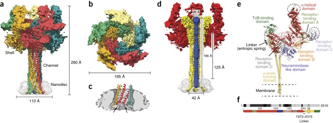
wild type and mutant TcdA1 proteins. (PDF 4108 kb) CRYO-EM MAP OF TCA IN ITS PORE STATE EMBEDDED IN NANODISCS. The cryo-EM map of TcA from Photorhabdus luminescens, colored by subunits and

filtered according to local resolution (see Supplementary Fig. 1 for details), is rotated to show the overall structure and zoomed in on representative regions, in particular an α-helix and

a β-strand. Last, the molecular model of the linker (entropic spring) is shown superimposed with the respective cryoEM density. (MOV 11019 kb) CONFORMATIONAL CHANGE OF THE TRANSMEMBRANE

DOMAIN FROM PREPORE TO PORE STATE. The video focuses on the conformational changes of the transmembrane domain showing the membrane-induced opening of the pore. The narrowest site of the

prepore lumen (Tyr 2,163) is shown in sticks (MOV 6225 kb) INTERACTION BETWEEN THE TRANSMEMBRANE REGION OF TCA AND THE LIPID HEAD GROUPS. The animation includes 0.5 μs of simulation,where

the lipid head groups recurrently intercalate between the helices of the protein. We highlighted the intercalated lipids for a representative frame located around the middle of the

simulation. (MOV 22963 kb) SYRINGE-LIKE INJECTION AND CHANNEL OPENING MECHANISM. The video shows a simplified model of the syringe-like injection, membrane penetration and channel opening,

obtained after morphing between the structure of TcA in the prepore and the pore state. It should be noted, that a structure of a possible intermediate state (with the toxin inserted in the

membrane but the channel in the prepore state), as shown in this animation, is not available yet. (MOV 3140 kb) CONFORMATIONAL CHANGE BETWEEN PREPORE TO PORE TCA PROTOMER. The video shows a

morph between the structures a TcA protomer in the prepore and pore state. The conformational changes of the entropic spring are highlighted. (MOV 1970 kb) REPRESENTATIVE TRAJECTORIES ALONG

THE LINKER EXTENSION FREE ENERGY CALCULATIONS. States near the pore, and prepore extensions, as well as an intermediate state are shown. The blue spheres show the atoms used to measure the

end-to-end distance of the molecule. For guidance, the positions of the trajectories along the free energy profile are highlighted. (MOV 3454 kb) MEMBRANE DEFORMATION DURING THE

COARSE-GRAINED MD SIMULATIONS OF MEMBRANE PENETRATION. The trajectories for each of state shown in Fig. 5 are included. For guidance, the position of the windows along the free energy

profile is indicated with an arrow. (MOV 11480 kb) RIGHTS AND PERMISSIONS Reprints and permissions ABOUT THIS ARTICLE CITE THIS ARTICLE Gatsogiannis, C., Merino, F., Prumbaum, D. _et al._

Membrane insertion of a Tc toxin in near-atomic detail. _Nat Struct Mol Biol_ 23, 884–890 (2016). https://doi.org/10.1038/nsmb.3281 Download citation * Received: 06 May 2016 * Accepted: 26

July 2016 * Published: 29 August 2016 * Issue Date: October 2016 * DOI: https://doi.org/10.1038/nsmb.3281 SHARE THIS ARTICLE Anyone you share the following link with will be able to read

this content: Get shareable link Sorry, a shareable link is not currently available for this article. Copy to clipboard Provided by the Springer Nature SharedIt content-sharing initiative